a certain range of the nominal VDD value to guarantee the reliable power delivery. ... gradient optimization, we develop a new search step scheme to speed up the ..... our iCG optimization engine to have the individual partition decap budget ...
IEEE TRANSACTIONS ON COMPUTER-AIDED DESIGN OF INTEGRATED CIRCUITS AND SYSTEMS, VOL XX, NO. XX, DECEMBER 200X
1
Partitioning-Based Approach to Fast On-Chip Decoupling Capacitor Budgeting and Minimization Hang Li, Student Member, IEEE, Jeffrey Fan, Student Member, IEEE, Zhenyu Qi, Student Member, IEEE, Sheldon X.-D. Tan, Member, IEEE, Lifeng Wu, Yici Cai, Xianlong Hong Fellow, IEEE
Abstract— This paper proposes a fast decoupling capacitance (decap) allocation and budgeting algorithm for both early stage decap estimation and later stage decap minimization in today’s VLSI physical design. The new method is based on a sensitivitybased conjugate gradient (CG) approach. But we adopt several new techniques, which significantly improve the efficiency of the optimization process. First, we propose an efficient search step scheme to replace the time-consuming line search phase in conventional conjugate gradient method for decap budget optimization. Second, instead of optimizing an entire large circuit, we partition the circuit into a number of smaller subcircuits and optimize them separately by exploiting the locality of adding decaps. Third, we apply time-domain merged adjoint method to compute the sensitivity information and show that the partitioning-based merged adjoint method leads to better results than the flat merged adjoint method with the improved search scheme. Experimental results show that the proposed algorithm achieves at least 10X speed-up over the similar decap allocation methods reported so far with similar budget quality, and a power grid circuit with about one million nodes can be optimized using the new method in half an hour on the latest Linux workstations.
arises from resistive and inductive effect, intentionally adding decoupling capacitance (decap) between power and ground buses or between power/ground buses and substrate is the most efficient way. As shown in Fig. 1, decaps provide a reservoir of current that is instantly available for the near switching components to remove spikes and glitches in the power rail. Since on-chip decaps are typically manufactured using MOS transistors, and excessive on-chip decaps could cause more leakage power, low yield and lower resonant frequency [1], the total decap area should be added in an area-efficient way.
Index Terms— Decoupling Capacitor, IR drop, On-Chip Power/Grid Networks
I. I NTRODUCTION Power integrity has become the most insidious issue in nowadays deep sub-micron and nanometer VLSI regime. IR drop is caused by device switching current flowing through the parasitic power/ground network. A supply voltage (VDD/GND) variation throughout the entire chip will occur, which will lead to adverse impact on chip performance, longer path delay, or even logic failure. With the reduced noise margin and increased switching frequency as technology scales, it is required to confine the supply voltage fluctuation within a certain range of the nominal VDD value to guarantee the reliable power delivery. For removing dynamic IR drop which Some preliminary results of this paper appeared in Proc. Design Automation Conference (DAC’05), Proc. Int. Symposium. on Quality Electronic Design (ISQED’05) [11], [14] Hang Li, Jeffrey Fan, and Sheldon X.-D. Tan are with Department of Electrical Engineering, University of California, Riverside, Riverside, CA 92521 USA (e-mail: {hli,jfan,stan}@ee.ucr.edu) Lifeng Wu is with Cadence Design Systems Inc. Yici Cai and Xianlong Hong are with Department of Computer Science and Technology, Tsinghua University, Beijing, 100084, China USA (e-mail: {caiyc,hxl-dcs}@mail.tsinghua.edu.cn) This work is funded by NSF CAREER Award CCF-0448534, NSF grant OISE-0451688, UC MICRO #04-088 via Cadence Design System Inc. The work of Y. Cai and X. Hong is funded by Hi-Tech Research & Development (863) Program of China 2004AA1Z1460 and the National Natural Science Foundation of China (NSFC) 60476014.
Fig. 1.
The model of power grid networks.
Budgeting decap in an area-efficient way, however, is a difficult task due to prohibitive analysis costs of power/grid (P/G) networks with millions of nodes and extracted onchip and off-chip RLC components in modern VLSI design. Mathematically, optimal decap allocation is a nonlinear optimization problem and many existing approaches [7], [18] use sensitivity-based optimization methods to solve the problem. To compute the sensitivity, transient simulations of the whole P/G networks have to be carried out at every optimization step. Given the fact that the transient simulation of P/G networks with millions of nodes is already an extremely time-consuming task, the CPU and memory cost of the optimization method that uses transient simulations as the internal loops will be prohibitive. Recent study [7] shows that allocating decaps for a P/G grid with about one million nodes will take about 10 hours in modern workstations with improved simulation techniques. Given the increasing sizes of P/G networks, existing decap budgeting techniques do not scale well for future VLSI onchip power distribution network design and verification. An alternative approach based on multigrid concept was proposed by Wang and Marek-Sadowska in [21]. But this
IEEE TRANSACTIONS ON COMPUTER-AIDED DESIGN OF INTEGRATED CIRCUITS AND SYSTEMS, VOL XX, NO. XX, DECEMBER 200X
method is limited to the regular-mesh or regular-mesh-like P/G structures. This method exploits the geometrical multigrid method for sizing the widths of P/G wires and allocating decaps. At the reduced mesh level, Sequential Quadratic Programming is still used, where sensitivity is computed by adjoint method only. But for the non-mesh structured P/G networks, this method may not work due to the use of geometrical multigrid idea. Also during the re-mapping process (map the decap results from high level grid to low level grids), the method requires that all the widths of P/G wires are same in a P/G strip. Otherwise, the re-mapping process will not guarantee the existing of the solution at the low level. Actually this will not be satisfied for the actual industry P/G network circuits. Also, if there are many C4 pads (voltage sources), the reduction ratio will be reduced, so does the efficiency of this method. In short, the multigrid based method has many restrictions and limitations. In this paper, we propose a general fast decap allocation and budgeting algorithm in solving large power grid circuit, which is modeled as RLC networks considering both on-chip and offchip parasitics. The new method is based on the sensitivitybased conjugate gradient methods. Our contributions include: (1) Instead of doing line search at every step in conjugate gradient optimization, we develop a new search step scheme to speed up the optimization process; (2) Based on the local effect of adding decap to reduce IR drops, we partition the whole circuit into a number of sub-circuits and optimize them individually. A noise-aware partition scheme is proposed to perform the required partitioning. (3) We applies the timedomain merged adjoint network method in [7], [18] for sensitivity calculation in the partitioning-based optimization framework. We show that combining the proposed partitioning scheme with the merged adjoint method leads to much faster optimization process with similar solution quality given by the flat CG using the merged adjoint method [7], [18]. The combination of our new optimization algorithm and partition scheme significantly improves the analysis speed for very large power/ground circuits even on a single CPU workstation. We notice that adding decaps alone may not solve all the voltage drop problems in power/ground grids. Our recent study by considering leakage of decaps [8] shows that decap leakage can lead to more decap areas for the same noise reduction effects. In this case, considering both wire sizing and decap allocations are better solutions [8]. The proposed method can be used to optimize the power/ground networks before or after the wire sizing step, as leakage currents are mainly DC currents and can be optimized more efficiently by wire sizing. We notice that the time-domain merged adjoint method has been used for transistor sizing [6] and then later applied to the decap optimization in [7], [18]. But we show in this paper that with the proposed partitioning scheme, the merged adjoint method works better than the simple application of the merged adjoint method in the CG optimization framework. The rest of the paper is organized as follows: Section II briefly reviews existing sensitivity-based decap budgeting algorithms. In Section III, we describe our new algorithm, with theoretical analysis regarding to time efficiency. Section IV gives description of a graph-based partition algorithm in
2
dealing with special decap situation. The experimental results are summarized in section V to verify our method, with conclusions in section VI. II. R EVIEW
OF
P REVIOUS D ECAP O PTIMIZATION A LGORITHMS
Existing on-chip decap budgeting algorithms basically fall into two categories. In [2], [12], [16], [17], the current pattern around hot spots (where violation of IR drop occurs) is derived and the amount of electric charge needed to supply that current demand is estimated. To obtain an optimal decap budget, a critical step for these methods is the precise estimation of voltage drops, which unfortunately proves to be difficult for practical P/G networks without simulation.
Fig. 2.
Illustration of IR drop violations.
Another category is sensitivity-based approaches based on actual circuit simulation, which is a more accurate and wellaccepted method. Fig. 2 gives an illustration of VDD fluctuation of a node within one clock cycle [18]. The violation area at node j is defined as: Z T gj (c1 , ..., cn ) = max(Vmin − vj (t), 0)dt (1) 0
which equals to the shaded area below a certain VDD threshold in the graph. The sensitivity of decap added at node i in contributing to remove this violation area at node j is: sij =
∂gj (c1 , ..., cn ) ∂ci
(2)
where ci is the decap value added at node i, and n the number of nodes where decaps can be added. If we allow all circuit nodes to be candidates for adding decaps, n equals to the number of circuit nodes. The adjoint network method is the conventional way to calculate this sensitivity, which requires two full circuit simulations, one for the original network and the other for the adjoint network. The sensitivity for capacitive elements can then be expressed as: Z T 0 sij = vi,j (T − t) × v˙ i (t)dt, ( i = 1, 2, ..., n) (3) 0
where v˙ i (t) is the derivative of voltage waveform at node i in 0 the original network, and vi,j (T − t) is the waveform at node i in the adjoint network under unit step current excitation at violation node j.
IEEE TRANSACTIONS ON COMPUTER-AIDED DESIGN OF INTEGRATED CIRCUITS AND SYSTEMS, VOL XX, NO. XX, DECEMBER 200X
In previous work [18], a sensitivity-based algorithm is developed to optimize the allocation of decaps in a standard cell design format. In its problem formulation, it minimizes the following objective function m X
min
gj (c1 , ..., cn )
j∈Nvio
where Ndecap is the set of all the decap nodes and Nvio is the set of all the violation nodes. The new objective function is solved by traditional conjugate gradient (CG) method within each optimization iteration. The weighting factor α in (5) is used to balance the two terms, and will keep changing in each CG iteration. However, such balance could be misleading since the optimization direction may be decided by the value of α rather than the sensitivity of each decap value to the objective function. Improper α will cause extra line searches, or even optimization failure. What’s more, each line search during CG optimization also requires the evaluation of the objective function at the cost of a full transient simulation, which renders the algorithm inefficient and unreliable. In this paper, we present our improved conjugate gradient (iCG) algorithm, which takes the advantage of the fast sensitivity computation in [7], while avoids the ambiguity of the old optimization objective and the inefficient line search phase. III. I MPROVED C ONJUGATE G RADIENT A LGORITHM In our new iCG algorithm, we follows the similar problem definition in [18]. Specifically we formulate the optimization problem as:
gj (c1 , ..., cn )
ci ≤ d i ,
(4)
which is the sum of the violation areas of all the violation node. The constraints are the lower and upper bounds of the decap values and the total decap areas in each row (the total white space in the layout) for each decap node. n is the number of violation nodes. Then the problem is solved by a quadratic programming solver. The iteration continues until all violations are eliminated. For the gradient computation, adjoint network method in Eq. (3) is used to obtain the sensitivity value of the objective function to each decap value. The sensitivity of every violation node with respect to every decap node is computed within each iteration. Therefore, the time complexity is approximately O(n1.5 lmh), where m is the number of violation nodes, l the number of sampling time points, and h the number of optimization iterations. The term h depends on the convergence rate of the optimization method, and n1.5 is the typical time complexity for solving sparse n × n matrices [19]. It is clear that the speed of this algorithm depends on the number of violation nodes, and will become intolerable for extremely large circuits. Recent work [7] improved the sensitivity calculation by applying the time domain merged adjoint network method, which will be covered later in the next section. The decap area is incorporated into the objective function as: X X gj ) (5) ( ci ) + α(
m X
(6)
j=1
subject to constraints
j=1
i∈Ndecap
Objective function
3
di ≥ 0
(7)
where m is the number of violation nodes, and n the number of decap nodes. di is the maximum decap allowed at node i, a parameter decided by the available layout white space around node i. Notice that the upper bounds di at different nodes may not independent as shown in the standard cell based layout [18] since total decap areas may be fixed. But those dependences can be easily considered in our algorithm as those geometry related constraints are explicitly checked and enforced during the optimization process. Although we do not put decap areas in the objective function as in [7] because they cause many problems in CG based optimization framework as discussed in previous section, we do minimize the decap area implicitly in the CG optimization framework by following the CG direction in each CG iteration step and later performing the proposed binary line research (to be discussed later). Note that the decap budgeting problem defined in Eq.(6) and Eq.(7) can be used in early floor-planning stage for decap budget estimation, where di is the available white-space that can be used for adding decaps. The same optimization formulation can also be used in the later stage of physical design to minimize the existing decap budget, since some decaps are placed heuristically in the previous design stage. The di then represents the decap value already allocated at node i. As mentioned in section II, the sensitivity of the objective function (6) with respect to each decap value can be computed by the merged adjoint network method. In conventional adjoint network, a unit step current source is placed at each violation node when calculating the sensitivity described in Eq.(2). However, since all the adjoint networks for each violation node share the same topology, we may combine the step current sources together based on circuit superposition. And the sum of all the decap sensitivities would turn into: Z T m X 0 sij = (vi,all (T − t)) × v˙ i (t)dt ( i = 1, 2, ..., n) (8) j=1
0
0 (T − t) is calculated from the merged adjoint where vi,all network with combined step current sources. The merit of this method can be observed immediately since Pm m X ∂ j=1 gj (c1 , ..., cn ) sij = (9) ∂ci j=1
where the right-hand-side is just the sensitivity of the objective function we need in our problem formulation. Therefore, all the decap’s sensitivity to the objective function can be calculated in only two transient simulations, which greatly improves the efficiency of the algorithm. Although the merged adjoint method can significantly reduce the number of full circuit transient simulations, a number
IEEE TRANSACTIONS ON COMPUTER-AIDED DESIGN OF INTEGRATED CIRCUITS AND SYSTEMS, VOL XX, NO. XX, DECEMBER 200X
of simulations are still needed at each step in the CG method. The reason is that the direct application of the CG method in [7] requires evaluations of the objective function at different points along the current gradient direction to find the minimum cost in the objective function. But the cost of simulation in this line search phase is expensive, and could offset the efficiency gained by the merged adjoint method. In order to avoid this, we develop a simple, yet efficient search step computation method. The method is based on the observation that the step size in each search direction can be simply determined by computing the maximum decap value allowed on one or some nodes under this search direction. In other words, we determine the maximum step we can take in current direction, and set each decap values according to this step. We will continue to do so until violation criterion has been met. One problem with such a maximum-allowable-step scheme is that it may overestimate the decap areas. To alleviate this problem, a binary search will be performed to find the best step such that all violations are just removed and decap areas are minimized. The main difference of our method from the traditional CG method is that we only need to do binary search just once in the entire optimization process, which is in contrast to the traditional CG method, where the line search is carried out at every CG step during optimization. The new proposed decap budgeting algorithm can be illustrated in Fig. 3, which has two stages. First, the existence of solution is checked in the present direction computed by the CG method. Then a solution is located by binary searches. Within each CG iteration, only two transient simulations are needed for gradient computation. So the time complexity of the algorithm is about O(n1.5 l(h+r)). Again, n is circuit node count, l is the number of time points and h is optimization iteration number. r denotes the number of steps in which binary search is attempted. Time complexity of [7] is derived in the original paper and can be expressed as O(n1.5 lh(2 + r0 )), where all variables are defined as above except r 0 , which is the number of line searches in each iteration. Usually h, r 0 and r are all within the same order of magnitude. So the proposed algorithm can be expected to be much faster as we only do the binary (line) search once and avoid the hr 0 term in the time complexity. Compared with decap algorithm in [18], the proposed method also leads to a great run time reduction, as it is independent with the number of violation nodes. Also, the faster convergence and less computation cost of conjugate gradient than quadratic programming contributes to the time efficiency as well. IV. PARTITIONING -BASED A NALYSIS OF P/G AND D ECAP B UDGETING
NETWORK
Accurate decap budgeting relies heavily on repeated transient analysis of the entire power grid. With a full-chip power grid model consisting of millions of nodes and elements, the burden on computation and memory storage during optimization is huge. For decap optimization, which asks for full circuit simulation at each time point, it is desirable to reduce the problem size of analysis by partitioning the large circuit into
4
Solve input circuit & Establish violation node set
Violation requirement satisfied ?
Y
N Store waveform for all nodes
Construct merged adjoint network; Convolve for sensitivities
Compute conjugate gradient direction; Obtain the maximum step
Update all decaps with this step; Do transient simulation with updated decap values
Halve the step; Update decap values; Do transient simulation with updated decap values
Y
Violation requirement satisfied ?
N Take the previous decap value
Finalize decap budget with the smallest possible step obtained
Fig. 3.
The proposed decap budgeting optimization flow.
several smaller sub-circuits, and optimize decap budget of each partition separately, or even in parallel. The partitioning-based strategy is also supported by the fact that adding decap to remove IR drop violation is a local effect. Normally, the violation occurs in the center or a certain area on the chip. For the emerging flip-chip packaging technology, this local effect becomes more prominent [4]. The number of violation nodes compared to the total circuit node number is also supposed to be small. Otherwise, the entire power network should be re-designed. For each violation node, the most effective decap locations are always the nodes close to it. Thus we should expect only a few good decap candidate locations through the entire chip for each violation node. A. General Partition Algorithm In our paper, we use the graph-based multilevel minimum cut algorithm for partitioning task [9], which provides an extremely fast speed on large graph sizes, where a graph with one million vertices can be processed roughly within one minute. This ensures that the partition phase will not bottleneck our entire partitioning-based optimization flow. Specifically, we first convert the power grid netlist in SPICE format to the graph file style accepted by METIS. Then, we read in the output file generated by METIS, and create each individual partition’s netlist file. These files are processed serially by our iCG optimization engine to have the individual partition decap budget result. The final decap budget will simply be the combination of all partition’s budgets.
IEEE TRANSACTIONS ON COMPUTER-AIDED DESIGN OF INTEGRATED CIRCUITS AND SYSTEMS, VOL XX, NO. XX, DECEMBER 200X
TABLE I D ECAP BUDGET COMPARISON BEFORE / AFTER PARTITION Subcircuit Name 1 2 17 18
Original Budget 1.00 1.00 1.00 1.00
w/ boundary budget deviation 1.11 11.2% 0.77 -22.9% 1.22 22.6% 1.38 38.8%
w/o boundary budget deviation 1.48 48.1% 1.64 64.0% 1.23 22.6% 1.72 71.7%
A direct use of partitioning without considering the IR drop violation could have adverse impacts on the entire decap optimization. Because we should avoid putting violation nodes as the boundary nodes, whose node voltage can’t be reduced by adding decaps, since boundary node voltages are treated as independent voltage sources as discussed below. B. Boundary Condition for Sub-circuits For each sub-circuit, we need to consider the influence of other sub-circuits on its decap budget optimization. We call this boundary condition of the sub-circuit. If boundary condition for each individual partition is not considered, the decap budget will be conservative compared to the one presented in the original netlist. The reason is that the subcircuit, as opposed to the full circuit, confines currents to flow in a smaller area, instead of the global P/G network. As consequence, more currents (due to smaller resistance to true ground) occur in the same area after partitioning. These over-estimated currents will cause greater IR drops than actual ones. To solve this problem, we keep the boundary node waveforms in piece wise linear (PWL) form derived from a full circuit transient simulation at the beginning of the optimization. In this way, the voltage waveforms are the same even when each sub-circuit is simulated independently. In Table I1 , a circuit with 240K nodes is partitioned into 20 pieces. Decap budgets are compared between several subcircuits with PWL boundary conditions and the ones without. Deviation is calculated as the difference between the budget of each sub-circuit and the budget of the same sub-circuit in the original circuit optimization. We notice that there are only 4 sub-circuits containing violation nodes, and the deviation of the simple partition budget without the boundary conditions is much greater than the one with boundary conditions. C. Noise-aware Partitioning (NAP) Keeping boundary node voltage as independent voltage sources introduces another problem. The violation nodes may appear as the boundary node in each partition, and there is no way to reduce voltage drop of the PWL voltage source at the violation node by adding decaps. Therefore we should explicitly avoid putting violation nodes into the boundary node set during partitioning. This can be easily implemented by assigning a relatively heavy edge weight incident on each 1 In this table, as well as in other tables in the rest of this paper, the decap budget for the comparison of CG, iCG, and later partitioning-based iCG algorithms, are scaled values such that the decap values given by CG using the merged adjoint method is 1.0
5
violation node, as well as the nodes adjacent to them. Since the partition algorithm attempts to minimize the total cut weights on the boundary, those weighted violation node edges have a very low possibility to be cut. Another issue is that we should keep the good decap candidate nodes for violation nodes in the same sub-circuit. Otherwise, it will be more expensive to reduce the IR drops of the violation nodes by using less effective nodes available in a sub-circuit. To this end, we need to consider adding decap range for violation nodes during partitioning. The current sources at the violation nodes typically are the cause of IR drop violation, and will be assigned into one sub-circuit along with all the nodes they are directly connected to or in nearby locations. To achieve this, we can assign a relatively small vertex weight to each violation node containing current source, as well as a pre-defined radius, within which the nearest nonviolation nodes close to it are also given the same weight. Given the fact that the partitions should be balanced in terms of each partition’s total vertex weight, the violation nodes will be aggregated with a host of nearby non-violation decap candidate nodes.
Fig. 4.
Example of noise-aware partition scheme.
Fig. 4 gives a simple example of above proposed partition scheme. We observe that the violation nodes 16 and 21 are easily separated into two partitions without any differentiation between them and the non-violating ones. After we add larger weights on the edges around them, they are captured into one partition. If we further assign a smaller vertex weight to them, as well as the ones in adjacent to them, which are node 10, 15, 17, 20 and 22, more surrounding nodes will go with node 16 and 21 into the same sub-circuit, which is exactly what we expected. By using this noise-aware partition (NAP) scheme, we did the test on previous 240K circuit again. The original budget refers to the budgets obtained in the flat run of the optimization
IEEE TRANSACTIONS ON COMPUTER-AIDED DESIGN OF INTEGRATED CIRCUITS AND SYSTEMS, VOL XX, NO. XX, DECEMBER 200X
6
TABLE II Solve input circuit; Establish violation node set
D ECAP B UDGET C OMPARISON UNDER NAP Subcircuit Name 4 5 14
Original Budget 1.0 1.0 1.0
Partitioned Budget 0.80 0.63 1.01
Transfer netlist into graph file format with current decap values; Feed into partition solver
Find all boundary nodes; Extract their PWL form; Establish partition set
for each subcircuit. We observe that the results in Table II show that the new partition budget is very close to or even smaller than the one from the original circuit. In Table II, Original Budget is obtained by using CG with the merged adjoint method. The reason is related to the merged adjoint method, which leads to worse results compared to conjugate gradient method using the sensitivities of individual violation node area (without using the merged adjoint method). The merged adjoint method computes the sensitivity of the objective function, which is sum of all the violation node areas, with respect to each specific decap instead of sensitivities with respect to each individual violation node area. As a result, the CG with the merged adjoint method will lead to worse results than the CG using the sensitivities of individual violation node simply because the later method can use each decap to its maximum effects for reducing voltage drops while the former method does not have the flexibility to fine tune the each decap’s contribution to a specific violation node. Our recent study by using sequence of linear programming method for decap budgeting shows that using individual sensitivities of violation decap nodes can get much better quality than the merged adjoint method [13]. On the other hand, the partitioning scheme tends to reduce the adverse effects of the merged adjoint method as partitioning tries to make the sensitivities to be limited to the violation nodes in each partition. In the extreme case, each partition has just one node, we go back to the non-merged sensitivity computation case in which we should have the best result in this regard. But in this case, another problem will kick in: very large partition number will lead to no solution for our iCG optimizer due to the limited decap nodes in each partition. Therefore, for a certain range, the decap budget from larger partition number will result in better optimization results. Although partition helps to improve the optimization results in CG algorithm using the merged adjoint method. It also degrade the optimization quality as it makes some violation nodes harder to optimize, which will be explained in experimental section. As a result, the net effect of using partitioning scheme is the increased efficiency of the optimization with the similar quality of the CG method using merged adjoint method [7]. Note that for the power/ground networks with many C4 pads, the C4 region can be used as natural partitions as shown in [4]. In this case, no explicit partitioning is required and the partitioning-based decap optimization can be done naturally in C4 power/ground networks.
Generate each partition netlist with PWL information included
Y Partition set is empty?
N Call iCG solver to do individual partition optimization
N
Combine updated decap values; Generate new netlist file
Solve new circuit with updated decap values
Y Violation criterion met?
N Decrease previous partition number
Finalize decap value at each node in the optimized result
Fig. 5.
The partitioning-based optimization flow.
D. Partitioning-based Decap Optimization Flow The whole partitioning-based optimization flow is given in Fig. 5. It performs only two full circuit transient simulations, one at the very beginning to report all the violation nodes and record the original boundary node waveform, another in the last to verify the optimization result. Compared to many full simulations carried out in a flat run mode, the time overhead from these two full circuit simulations becomes less significant. The rest of simulations will be conducted on each sub-circuit only, which are much faster than full circuit simulation even done sequentially. We assume a number of N partitions (sub-circuits) with approximately the same amount of nodes in each partition. Since the partitions are processed sequentially in our experiment, and parameters l, h, and r won’t change too much with partitioning, the new time complexity becomes N [(
[n1.5 l(h + r)] n 1.5 √ ) l(h + r)] = N N
(10)
Therefore, the time complexity of partitioning-based optimization algorithm will decrease with the square root of the number of partitions. However, the number should not be very large either. Because a very small sub-circuit could result in
IEEE TRANSACTIONS ON COMPUTER-AIDED DESIGN OF INTEGRATED CIRCUITS AND SYSTEMS, VOL XX, NO. XX, DECEMBER 200X
no solution of optimization due to reduced decap candidate positions. In case of no solution is found in the sub-circuits, we will halve the partition number, and re-run the whole algorithm again for a relaxed partition area. Since we snapshot the IR drop violation by defining an effective area for adding decap in partitioning, the optimization effect is supposed to be guaranteed when all the partitions are combined together. If parallel computing is allowed, the time complexity can be further reduced to [n1.5 l(h + r)] (11) N 1.5 since there is no communication needed between different partitions during decap optimization. V. E XPERIMENTAL R ESULTS We implement our proposed algorithm in C++. All experiments are carried out on a Linux PC with dual 3.0Ghz Xeon CPUs and 2GB memory. All test circuits are generated by the authors with realistic parameters for R, C and current sources based on industry designs. The off-chip inductive parasitic effects are also considered. Some figures are exaggerated in order to test the versatility of our algorithm. For each test case, we artificially set the power noise level such that the number of violation nodes presented in the circuit is within 20% range of the total node count. Keep in mind that we can not count solely on adding decaps to eliminate all IR drop violations, and a huge amount of violation is not reasonable for decap solution. We first compare our method with [7] for small circuits without partitioning. To make comparison possible, we implement [7] in such a way that before each line search, an explicit attempt to bracket the minimum is made, and if the minimum is found to lie at the start of the line, α is augmented. In this way, we avoid the problem mentioned in section II and make the algorithm robust enough for all our tests. Table III summarizes the comparison, where CG1 denotes the method in [7] and CG2 denotes our iCG method. Columns 1, 2, 3 represent circuit names, total node numbers, and violation node numbers respectively. Parameters including voltage drop tolerance, the maximum decap at each node can be specified by users and are the same for both methods. The last column compares total optimization CPU time for the two algorithms. For all these circuits, violation elimination requirement is successfully achieved after both decap optimization. The CPU time efficiency of the proposed method is usually more than 10 times faster than the method in [7]. We also notice that the new method does trade some qualities for speed-up. We apply our partitioning-based optimization algorithm for larger power grid circuits. As shown in Table IV, comparisons are made between the budget and CPU time of the flat CG1, CG2, and the partitioning-based CG2 algorithm. Please note that the CPU time includes initial simulation time and partition time. The circuit sizes range from 240K to 1M nodes. While CG1 is still capable of solving ckt6 and ckt7, it fails to work on 800K and 1M cases. The main reason arises from the memory limitation (we have 2G memory in our Linux
7
workstation) for LU decomposition and waveform storage in sensitivity calculation during each transient simulation. CG2 suffers the same problem when doing the optimization flatly. The partitioning-based algorithm, on the other hand, can handle these cases very easily. As can be seen from Table IV, the partitioning-based algorithm optimizes all circuits successfully, and the budget achieved is comparable, or even smaller than the flat optimization runs. The time advantage is also impressive. The circuit with one-million nodes can be optimized in about half a hour, as opposed to a 10-hour run time in [7] for the same circuit volume 2 . Another thing that needs to be pointed out is that we simulate the circuits based on direct LU decomposition, while a structure level reduction technique is applied in [7] for the simulation on an actually smaller circuit size. The time efficiency of the algorithm is therefore more obvious. Since the efficiency of our proposed method depends on the linear solver used, any speedup techniques like hierarchical approach [22], multigrid methods [10], iterative methods [3], model reduction methods [5], [20] and random walk based algorithm [15] can be used to speed up and increase the capacity of the proposed method.
Fig. 6. Comparison of decap budget and CPU time between different partition sizes. .
We also notice that the difference among various partition sizes. For each example, the larger the partition number, the faster the speed as we projected. However, the decap budget experiences a variation. As an example of the 400K circuit illustrated in Fig. 6, with small partition numbers, the budget is over-estimated compared to flat-run result. The reason is that partitioning makes some violation node area harder to remove, as the available candidate decap nodes become less, due to the formation of sub-circuits and PWL voltage sources as the boundary. Those nodes typically are close to the boundaries of sub-circuits. Therefore, a larger decap value is added in each optimization iteration. But as partition number increases, the decap budget will drop as shown in Table IV. The reason actually has been explained in subsection IV-C. The results in Table IV further give the evidence that partitioning scheme can alleviate the adverse effect brought by the merged adjoint method. With larger partition numbers, we are more close to non-merged sensitivity computation case, so we will get better result. 2 The CPUs used in two papers are different (Intel Xeon versus Sun UltraSparc). It is difficult to scale the CPU times in terms of raw clock speeds.
IEEE TRANSACTIONS ON COMPUTER-AIDED DESIGN OF INTEGRATED CIRCUITS AND SYSTEMS, VOL XX, NO. XX, DECEMBER 200X
8
TABLE III C OMPARISON WITH THE Circuit
#Nodes
ckt1 ckt2 ckt3 ckt4 ckt5
88 336 1,233 12,673 89,496
#Vio Nodes 29 63 143 1,083 592
EXISTING
CG METHOD FOR P/G DECAP OPTIMIZATION
CG1 (existing) decap iter time(s) 1.00 8 2.3 1.00 10 15.2 1.00 10 132 1.00 8 1,995 1.00 5 7,241
CG2 decap 1.16 1.32 1.08 1.18 1.59
(proposed) iter time(s) 1 0.1 2 0.8 1 2.4 1 54 1 394
speedup ratio 23 19 55 37 18
TABLE IV C OMPARISON BETWEEN FLAT # of nodes 242,600 – – 421,320 – – 827,025 – – 1,004,960 – –
Circuit ckt6 ckt7 ckt8 ckt9
# of vio nodes 49,626 – – 26,843 – – 87,903 – – 67,105 – –
AND PARTITIONING - BASED DECAP OPTIMIZATION
CG1 budget time(s) 1.00 9,592 – – – – 1.00 15,555 – – – – N/A N/A – – – – N/A N/A – – – –
CG2 budget time(s) 1.29 1,746 – – – – 1.14 1,370 – – – – N/A N/A – – – – N/A N/A – – – –
partition no. 5 10 20 10 20 40 20 40 80 25 50 100
Partitioned CG2 budget time(s) 1.55 744 1.14 713 1.03 438 2.09 1,077 1.87 1,034 1.09 765 1.00 2,619 0.61 1,711 0.60 1,705 1.00 2,812 0.54 2,675 0.49 2,093
speedup ratio 13 13 22 14 15 20 N/A N/A N/A N/A N/A N/A
TABLE V C OMPARISON BETWEEN SEQUENCE LINEAR PROGRAMMING (SLP) AND Circuit ckt10 ckt11 ckt12 ckt13
ckt14
# of nodes 6,105 – – 29,425 – – 89,496 – – 123,280 – – – 536,705 – – –
# of vio nodes 206 – – 181 – – 251 – – 301 – – – 373 – – –
SLP (sen = 0.1) budget time(s) 1.00 470 – – – – 1.00 1,871 – – – – 1.00 6,911 – – – – 1.00 10,700 – – – – – – N/A N/A – – – – – –
SLP (sen = 1) budget time(s) 0.15 549 – – – – 0.10 2,123 – – – – 0.10 6,807 – – – – 0.10 10,557 – – – – – – N/A N/A – – – – – –
Since partitioning itself also degrades the decap allocation quality as discussed above, the total decap allocation quality, due to two effects, leads to similar quality given by the CG using the merged adjoint method, as shown in Table IV. But the proposed method can be much faster and more capable than the flat CG method. Also, the partition number should not be too large either. Otherwise, the number of decap nodes will become too small to have a solution for removing violating areas in the subcircuit. In such cases, we reduce the number of partitions and more partition iteration will be conducted as mentioned in Fig. 5, leading to a longer run time. Furthermore, we make a comparison between the partitioning-based decap optimization algorithm and Sequence
PARTITIONING - BASED OPTIMIZATION
partition no. 1 3 5 1 30 50 1 100 200 1 100 200 300 1 100 300 400
Partitioned CG2 METIS time(s) budget time(s) N/A 0.20 41 < 1.0 0.27 25 < 1.0 0.37 20 N/A 0.90 140 < 1.0 0.28 62 < 1.0 0.13 59 N/A 0.87 929 < 1.0 1.23 185 < 1.0 1.63 176 N/A 0.75 1,124 < 1.0 1.30 259 < 1.0 1.11 249 < 1.0 1.15 240 N/A 1.00 4,052 2.0 0.47 1,226 2.0 0.47 1,102 2.0 0.52 1,093
speedup ratio 11 19 24 13 30 32 7 37 39 10 41 43 45 N/A N/A N/A N/A
of Linear Programming (SLP) [13], as shown in Table V. In the SLP method, the sensitivities of each violation node voltage with respect to the all the decaps are computed (as a result, it becomes more expensive). So SLP enjoys the most flexibility during the decap optimization and it gives the better results. But the results of SLP strongly depends on a tuning parameter called sensitivity parameter [13]. Given a fixed sensitivity parameter (i.e. sen = 0.1), the experiment shows roughly 10X or more speed-up of the proposed method over the SLP method at the cost of decap quality in some circuits. Please note that the SLP method fails to solve the circuit with 500K nodes, while partitioning-based algorithm is able to solve the circuit in a timely manner. The increase of the sensitivity parameter will improve the quality of decap budget
IEEE TRANSACTIONS ON COMPUTER-AIDED DESIGN OF INTEGRATED CIRCUITS AND SYSTEMS, VOL XX, NO. XX, DECEMBER 200X
at the expense of slower speed in some circuits. Hence, the partitioning-based algorithm is more applicable when speed is the most concern for designers. One may notice that the METIS partition time is trivial in comparison to overall CPU time. VI. C ONCLUSIONS
AND
F UTURE W ORKS
In this paper, we have proposed a fast decap optimization solution, targeting at circuits with very large size. The combination of our proposed improved conjugate gradient algorithm and partitioning-based optimization scheme can efficiently optimize power grid circuits with million nodes in a timely manner. Our theoretical analysis on the time complexity shows that new algorithm outperforms most of the existing decap allocation algorithms. Practically, we show that combining the partitioning scheme with the merged adjoint method leads to faster optimization process without loss of the optimization quality compared to the flat CG algorithm with the merged adjoint method. Experimental results on a number of power grid circuits demonstrate that the proposed algorithm achieves roughly at least 10X speed-up or more over the similar decap allocation methods reported so far, and the power grid circuit with about one million nodes can be optimized in about half an hour on the latest Linux workstation. In the future, more efficient circuit simulation techniques, like hierarchical approach [22] and model reduction approaches [20] will be used to improve the transient simulation of the power/ground networks. Also, parallel simulation will be explored to further improve the efficiency of the decap budgeting algorithm. VII. ACKNOWLEDGEMENTS The authors would like to thank the anonymous reviewers of this paper for their comments and suggestions that helped improve this work. R EFERENCES [1] S. Bobba, T. Thorp, K. Aingaran, and D. Liu, “IC power distribution challeges,” in Proc. Int. Conf. on Computer Aided Design (ICCAD), 2001, pp. 643–650. [2] H. H. Chen and D. D. Ling, “Power supply noise analysis methodology for deep-submicron VLSI chip design,” in Proc. Design Automation Conf. (DAC), 1997, pp. 638–643. [3] T. Chen and C. C. Chen, “Efficient large-scale power grid analysis based on preconditioned Krylov-subspace iterative method,” in Proc. Design Automation Conf. (DAC), 2001, pp. 559–562. [4] E. Chiprout, “Fast flip-chip power grid analysis via locality and grid shells,” in Proc. Int. Conf. on Computer Aided Design (ICCAD), Nov. 2004, pp. 485–488. [5] E. Chiprout and T. Nguyen, “Power analysis of large interconnect grids with multiple sources using model reduction,” in Proc. European Conference on Circuit Theory and Design, Sept. 1999. [6] A. R. Conn, R. A. Haring, and C. Visweswariah, “Noise considerations in circuit optimization,” in Proc. Int. Conf. on Computer Aided Design (ICCAD), 1998, pp. 220–227. [7] J. Fu, Z. Luo, X. Hong, Y. Cai, S. X.-D. Tan, and Z. Pan, “A fast decoupling capacitor budgeting algorithm for robust on-chip power delivery,” in Proc. Asia South Pacific Design Automation Conf. (ASPDAC), Jan. 2004, pp. 505–510. [8] ——, “VLSI on-chip power/ground network optimization considering decap leakage currents,” in Proc. Asia South Pacific Design Automation Conf. (ASPDAC), Jan. 2005, pp. 735–738.
9
[9] G. Karypis, R. Aggarwal, and V. K. S. Shekhar, “Multilevel hypergraph partitioning: application in VLSI domain,” IEEE Trans. on Very Large Scale Integration (VLSI) Systems, vol. 7, no. 1, pp. 69–79, March 1999. [10] J. N. Kozhaya, S. R. Nassif, , and F. N. Najm, “A multigrid-like technique for power grid analysis,” IEEE Trans. on Computer-Aided Design of Integrated Circuits and Systems, vol. 21, no. 10, pp. 1148– 1160, Oct. 2002. [11] H. Li, Z. Qi, S. X.-D. Tan, L. Wu, Y. Cai, and X. Hong, “Partitioningbased approach to fast on-chip decoupling capacitor budgeting and minimization,” in Proc. Design Automation Conf. (DAC), 2005, pp. 170– 175. [12] M. Pant, P. Pant, and D. Wills, “On-chip decoupling capacitor optimization using architectural level current signature prediction,” in Proc. IEEE Midwest Symp. Circuits and Systems, 2000, pp. 772–775. [13] Z. Qi, H. Li, J. Fan, S. X.-D. Tan, Y. Cai, and X. Hong, “On-chip decoupling capacitor budgeting by sequence of linear programming,” in IEEE International Conference on Application Specific Integrated Circuits(ASICON), 2005, to appear. [14] Z. Qi, H. Li, S. X.-D. Tan, L. Wu, Y. Cai, and X. Hong, “Fast decap allocation algorithm for robust on-chip power delivery,” in Proc. Int. Symposium. on Quality Electronic Design (ISQED), 2005, pp. 542–547. [15] H. F. Qian, S. R. Nassif, and S. S. Sapatnekar, “Random walks in a supply network,” in Proc. Design Automation Conf. (DAC), 2003, pp. 93–98. [16] C. K. S. Zhao, K. Roy, “Decoupling capacitance allocation and its application to power-supply noise-aware floorplanning,” IEEE Trans. on Computer-Aided Design of Integrated Circuits and Systems, vol. 21, no. 1, pp. 81–92, Jan. 2002. [17] L. Smith, “Decoupling capacitor calculations for cmos circuits,” in Proc. IEEE Topical Meeting of Electrical Performance of Electronic Packaging, 1994, pp. 101–105. [18] H. Su, S. S. Sapatnekar, and S. R. Nassif, “Optimal decoupling capacitor sizing and placement for standard cell layout designs,” IEEE Trans. on Computer-Aided Design of Integrated Circuits and Systems, vol. 22, no. 4, pp. 428–436, April 2003. [19] J. Vlach and K. Singhal, Computer Methods for Circuit Analysis and Design. New York, NY: Van Nostrand Reinhold, 1995. [20] J. M. Wang and T. V. Nguyen, “Extended Krylov subspace method for reduced order analysis of linear circuit with multiple souces,” in Proc. Design Automation Conf. (DAC), 2003, pp. 247–252. [21] K. Wang and M. Marek-Sadowska, “On-chip power supply network optimization using multigrid-based technique,” in Proc. Design Automation Conf. (DAC), 2003, pp. 113–118. [22] M. Zhao, R. V. Panda, S. S. Sapatnekar, and D. Blaauw, “Hierarchical analysis of power distribution networks,” IEEE Trans. on ComputerAided Design of Integrated Circuits and Systems, vol. 21, no. 2, pp. 159–168, Feb. 2002.