Partitioning Multivariate Polynomial Equations via Vertex Separators ...

Partitioning Multivariate Polynomial Equations via Vertex Separators for Algebraic Cryptanalysis and Mathematical Applications Kenneth Koon-Ho Wong, Gregory V. Bard and Robert H. Lewis Abstract. We present a novel approach for solving systems of polynomial equations via graph partitioning. The concept of a variable-sharing graph of a system of polynomial equations is defined. If such graph is disconnected, then the system of equations is actually two separate systems that can be solved individually. This can provide a significant speed-up in computing the solution to the system, but is unlikely to occur either randomly or in applications. However, by deleting a small number of vertices on the graph, the variablesharing graph could be disconnected in a balanced fashion, and in turn the system of polynomial equations are separated into smaller ones of similar sizes. In graph theory terms, this process is equivalent to finding balanced vertex partitions with minimum-weight vertex separators. The techniques of finding these vertex partitions are discussed, and experiments are performed to evaluate its practicality for general graphs and systems of polynomial equations. Applications of this approach to the QUAD family of stream ciphers, algebraic cryptanalysis of the stream cipher Trivium and its variants, as well as some mathematical problems in game theory and computational algebraic geometry are presented. In each of these cases, the systems of polynomial equations involved are well-suited to our graph partitioning method, and constructive results are discussed. Mathematics Subject Classification (2000). 05C90, 11T71, 68R10, 94A60, 14G50. Keywords. balanced vertex partitions, graph partitioning, polynomial systems of equations, QUAD, Trivium, resultants, algebraic cryptanalysis.

1. Introduction There has been a long history of the use of graph theory in solving systems of equations. Graph partitioning techniques are applied to processes such as reordering variables in matrices to reduce fill-in for sparse systems [24, Ch. 7] and partitioning

2

Kenneth Koon-Ho Wong, Gregory V. Bard and Robert H. Lewis

a finite element mesh across nodes in parallel computations [54]. These techniques primarily focus on linear systems over the real or complex fields. In this paper, we apply similar graph theory techniques to systems of multivariate polynomial equations, and develop methods of partitioning these systems into ones of smaller sizes via their “variable-sharing” graphs. These techniques are intended to work over any field, finite or infinite, but are particularly suited to GF(2) for use in algebraic cryptanalysis of symmetric ciphers. Computing the solution to a system of multivariate polynomial equations is an NP-complete problem [7, Ch. 3.9]. A variety of solution techniques have been developed for solving these polynomial systems over finite fields, such as linearization, Gröbner bases, and resultants [8, Ch. 12], as well as recent ones such as SAT-solvers [9] and the Raddum-Semaev method [60]. Over the real and complex numbers, numerical techniques are also known including Gradient Descent, Newton’s Method, the Conjugate Gradient Methods and the Nelder-Mead Simplices Algorithm [6]. In addition, homotopy methods, also known as continuation methods, have become popular [3], but require the field to be ordered and complete. The graph partitioning method introduced in this paper could be a novel addition to the variety of methods available, principally as a preprocessor. From a multivariate polynomial system of equation, a variable-sharing graph is constructed with a vertex for each variable in the system, and an edge between two vertices if and only if those variables appear together in any equation in the system. Clearly, if the graph is disconnected, the system can be split into two separate systems of smaller sizes, and they can be solved for individually. However, even if the graph is connected, we show that it may be possible to disconnect the graph by eliminating a few variables by, for example, guessing their values when computing over a small finite field, and thereby splitting the remaining system. Over larger and infinite fields, we show how to perform the elimination with resultants. This suggests a divide-and-conquer approach to solving systems of equations. When the polynomial terms in the an system of equations are very sparse, we show that the system can usually be reduced to a set of smaller systems, whose solutions can be computed individually in much less time. In order for a partition of a system to be productive, the minimum number of variables should be eliminated, and the two subsystems must be approximately equal in size. This ensures that the benefit of partitioning the system is maximised. These conditions lead to the problem of finding a balanced vertex partition with a minimum-weight vertex separator on its variable-sharing graph, which is an NP-complete problem [39, 55]. Nevertheless, heuristic algorithms can often find near-optimal partitions efficiently [41]. In this paper, we apply this approach to polynomial systems arising from algebraic cryptanalysis of ciphers, and achieve significant advantages in attacking these ciphers. We also discuss some uses of graph partitioning to solve mathematical problems in game theory and computational algebraic geometry more efficiently. Section 2 introduces the necessary background in graph theory and graph partitioning. Section 3 shows how a system of polynomial equations can be split

Partitioning Multivariate Polynomial Equations via Vertex Separators

3

into ones of smaller sizes using graph partitioning methods. Sections 3.1 and 3.2 describe how the actual partitions can be found. In GF(2) polynomial systems, the values of the variables to be removed can be simply guessed, but in larger or infinite fields, we present an alternative method in Section 3.3. Section 4 provides results for some partitioning experiments and analyses the feasibility of equation solving via graph partitioning methods. We offer two cryptographic applications of vertex parititioning in Section 5. The first is a method whereby a manufacturer of a sparse implementation of QUAD, a provably-secure stream cipher family, could “poison” the polynomial system in the cipher, and thereby enable messages transmitted with it to be read by the manufacturer. Second, we present an algebraic cryptanalysis of Trivium, a profiled stream cipher in the eSTREAM project, as well as its reduced versions Bivium and Bivium-A, and discuss their vulnerability or resistance to graph partitioning methods. We also offer two applications to other branches of mathematics in Section 6. The first is finding the Nash equilibria in an 8-player game called “the cube game”. Normally, the equations for p-player Nash equilibria, without coalitions, are of degree (p − 1) [23, 63]. In this case, the equations are cubic, and the solution of them is greatly sped up by the techniques from this paper. The second is the Apollonius Problem, known to the Ancient Greeks but used in molecular chemistry [49]. Conclusions will be drawn in Section 7. Appendix A discusses the NP-completeness of finding balanced graph partitions. Some theorems guaranteeing the existence of balanced graph partitions for special graphs are given in Appendix B. An algorithm to convert from edge partitions to vertex partitions is given in Appendix C. Finally, some additional experimental results of graph partitioning are presented in Appendix D.

2. Preliminaries In this section, a brief introduction to graphs and graph partitioning is presented. For a detailed treatment on graph theory, see [36]. A graph describes a set of nodes and connections between them. Each node is called a vertex, and a connection between two nodes is called an edge. Let G = (V, E) be a graph with vertex set V and edge set E. Two vertices vi , vj ∈ V are connected if there is a path from vi to vj through edges in E. A disconnected graph is a graph where there exists at least one pair of vertices that is not connected, or if the graph has only one vertex. A graph G1 = (V1 , E1 ) with vertex set V1 ⊆ V and edge set E1 ⊆ E is called a subgraph of G. Given a graph G, subgraphs of G can be obtained by removing vertices and edges from G. Let G = (V, E) be a graph with k vertices and l edges, such that V = {v1 , v2 , . . . , vk−1 , vk }, E = {(vi1 , vj1 ), (vi2 , vj2 ), . . . , (vil , vjl )}. Removing a vertex vk from V forms a subgraph G1 = (V1 , E1 ) with V1 = {v1 , v2 , . . . , vk−1 }

4


and E1 = {(vi , vj ) ∈ E | vk ∈ / {vi , vj }}. We call G1 the subgraph of G induced by the vertex set (V − {vk }). Let G1 = (V1 , E1 ), G2 = (V2 , E2 ) be two subgraphs of G. G1 , G2 are considered disjoint if no vertices in G1 are connected to vertices in G2 . Clearly, the condition V1 ∩ V2 = ∅ is necessary. 2.1. Graph Connectivity The goal of partitioning a graph is to make the graph disconnected by removing some of its vertices or edges. The number of vertices or edges that needs to be removed to disconnect a graph is related to its vertex or edge connectivities respectively. Definition 2.1. The vertex connectivity κ(G) of a graph G is the minimum number of vertices that must be removed to disconnect G. The edge connectivity λ(G) of G is the minimum number of edges that must be removed to disconnect G. Clearly, a disjoint graph has vertex connectivity zero. On the other extreme, a complete graph Kn , where all n vertices are connected to each other, has vertex connectivity (n − 1). The removal of all but one vertex from Kn results in a graph consisting of a single vertex, which is considered to be disconnected. The following theorem relates graph connectivities with paths in the graph. Theorem 2.2 (Menger [53], 1927). If a graph has n vertex-distinct paths from any particular vertex to any other, then its vertex connectivity is at least n. Furthermore, if there are n edge-distinct paths then its edge connectivity is at least n. 2.2. Graph Partitioning The process of removing vertices or edges to disconnect a graph is called vertex partitioning or edge partitioning respectively. All non-empty graphs admit trivial vertex and edge partitions, where all connections to a single vertex are removed. This is obviously not useful for most applications. In this paper, we only consider balanced partitions with minimum-weight separators, in which a graph is separated into subgraphs of roughly equal sizes by removing as few vertices or edges as possible. 2.2.1. Balanced Vertex Partitions. More specifically, our primary focus of this paper is on balanced vertex partitions. Definition 2.3. Let G = (V, E) be a graph. A vertex partition (V1 , C, V2 ) of G is a partition of V into mutually exclusive and collectively exhaustive sets of vertices V1 , C, V2 , where V1 , V2 are non-empty, such that no edges connect vertices of V1 directly to vertices of V2 . The removal of C causes the subgraphs induced by V1 and V2 to be disjoint, hence C is called the vertex separator. For a balanced vertex partition, we require V1 and V2 to be of similar size. For a minimum-weight separator, we also require that C be sufficiently small. This is to ensure that the vertex partition obtained is useful for its applications, otherwise much of the original information would be lost.


5

Definition 2.4. Let G = (V, E) be a graph, and (V1 , C, V2 ) be a vertex partition of G with vertex separator C (see Definition 2.3). If max(|V1 |, |V2 |) ≤ α|V |, then G is said to have an α-vertex separator. The problem of finding α-vertex separators is known to be NP-hard. For more details, see Appendix A. Definition 2.5. Let G = (V, E) be a graph. If (V1 , C, V2 ) is a vertex partition of G, then define max(|V1 |, |V2 |) max(|V1 |, |V2 |) = β= |V1 | + |V2 | |V | − |C| to be a measure of balance of the vertex partition. Suppose the balance of a vertex partition of G into (V1 , C, V2 ) is β = α, then the partition also satisfies max(|V1 |, |V2 |) = α(|V1 | + |V2 |) ≤ α|V |, and hence the G has an α-vertex separator. Therefore, theorems that apply to α-vertex separators would also apply to vertex partitions with balance α. See [55] for more details of αvertex separators. Several theoerems governing the existence of α-vertex separators are presented in Appendix B. Figure 1 presents examples of balanced and unbalanced partitions, and their respective β values. The vertex separators C are circled, with the partitioned vertices V1 , V2 outside. The removal of the vertices in the separators disconnects the graphs. For a balanced partition, β should be close to 1/2.

original graph

unbalanced vertex partition (ȕ = 5/6)

balanced vertex partition (ȕ = 1/2)

Figure 1. Balanced and Unbalanced Vertex Partitions 2.2.2. Partitioning Algorithms and Software. Balanced edge partitioning is widely used in scientific and engineering applications, such as electric circuit design [62], parallel matrix computations [44], and finite element analysis [54]. Software packages are readily available for computing balanced edge partitions using a variety of algorithms [10, 13, 31, 37, 56, 57, 66]. On the other hand, balanced vertex partitioning has fewer applications, one of which being variable reordering in linear systems [24]. We are not aware of publicly available software that could be used for directly computing balanced vertex partitions with minimum-weight vertex separators. Therefore, we have chosen to use an indirect method to compute vertex partitions from edge partitions obtained by software. More details will be discussed in Section 3.

6


Unless otherwise stated, from here on we will only consider the problem of balanced vertex partitioning with minimum-weight vertex separators (sometimes simply referred to as vertex partitioning or partitioning) and its applications to solving systems of multivariate polynomial equations.

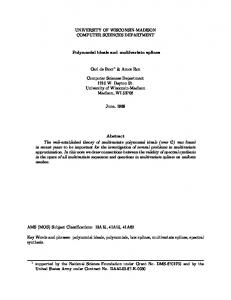
3. Partitioning Polynomial Systems In this section, our method for partitioning systems of multivariate polynomal equations by finding balanced vertex partitions of their variable-sharing graphs is described. Several methods for finding and using these partitions will also be discussed. Definition 3.1. Let F be the polynomial system f1 (x1 , x2 , . . . , xn ) = 0 f2 (x1 , x2 , . . . , xn ) = 0 .. . fm (x1 , x2 , . . . , xn ) = 0 of m polynomial equations in the variables x1 , x2 , . . . , xn . The variable-sharing graph G = (V, E) of F is obtained by creating a vertex vi ∈ V for each variable xi , and creating an edge (vi , vj ) ∈ E if two variables xi , xj appear together in any polynomial fk . Example 3.2. Suppose we have the following quadratic system of equations over GF(2), where the variables x1 , x2 , . . . , x5 are known to take values in GF(2). x1 x3 + x1 + x5 = 1 x2 x4 + x4 x5 = 0 x1 x5 + x3 = 0

(1)

x2 x5 + x2 + x4 = 0 x2 + x4 x5 = 1 The corresponding variable-sharing graph G and a balanced vertex partition is shown in Figure 2. The quadratic system can then be partitioned into two systems of equations with the common variable x5 as follows. x1 x3 + x1 + x5 = 1

x2 x4 + x4 x5 = 0

x1 x5 + x3 = 0

x2 x5 + x2 + x4 = 0 x2 + x4 x5 = 1

(2)

Partitioning Multivariate Polynomial Equations via Vertex Separators v3

v5

v4

v1

v3

vertex partition

v5

v4

v1

v2 G(V,E)

V1

7

v2 C

V2

Figure 2. Graph of quadratic system (1) and a vertex partition.

Since x5 ∈ GF(2), we can substitute all possible values of x5 into (1) and computing solutions to the reduced systems to give x5 = 0 ⇒ no solution x5 = 1 ⇒ x = (1, 0, 1, 0, 1) The solution obtained is the same as if we had directly computed the solution to the full system of equations. However, the systems have been reduced to having less than half the number of variables compared to the the original, at the cost of applying guesses to one variable. This method of guessing and solving will be used for the algebraic cryptanalysis of the Trivium stream cipher in Section 5. For simplicity, from here on we might use the terms for variables and vertices interchangeably to denote the variables in the polynomial systems of equations and their corresponding vertices in the variable-sharing graphs, provided there are no ambiguities. 3.1. Special Cases for Low Vertex-Connectivity Let G = (V, E) be a variable-sharing graph representing a polynomial system of equations. The special case of a disconnected graph with vertex connectivity κ = 0 for a graph G can be detected with a standard Depth-First Search (DFS). Mark each vertex “unvisited” initially, and mark it “visited” as the DFS progresses. If not all nodes are visited by the end of the DFS, then G is not connected. This has expected running time of Θ(|V |d) if the average degree of the graph is d. In this case, the polynomial system can be partitioned trivially, without a need to compute a vertex separator. The special case of κ = 1 can be detected by removing and restoring, one at a time, all vertices, and checking a DFS in each case. Likewise, κ = 2 can be detected by removing all possible pairs. The number of steps required to detect a vertex-connectivity of at most k is ¶ k µ X |V | i=0

i

|V |d ≈

(|V | + 1 − k/2) k!

k+1

d

,

8


where we have used µ ¶ µ ¶ µ ¶ a a a+1 + = , b b−1 b µ ¶ (a − n/2)n a , ≈ n! n

n ≪ a.

This approach also has the advantage of revealing the vertex separator. We call this Pseudo-Brute Force Search. For example, if |V | = 100, testing up to κ = 7 requires ¶ 7 µ X 100 = 17, 278, 988, 696 i i=0 depth-first searches. This may still be a feasible computation on distributed computing systems, since each DFS can be performed independently of each other. Since we desire a balanced partition, we can mark each subset of k or fewer vertices that partitions the graph, found during the search, with a difficulty number. The difficulty number should be the size of the largest connected component, since this will presumably be the hardest subsystem of equations to solve. At the conclusion of the search, we take the partition with the lowest difficulty number. This would assure that the optimal partition of all those possible can be discovered. 3.2. Heuristic Partitioning Algorithms The method above does not scale up to large graphs with high vertex connectivities, so other computational methods are required. While balanced partitioning is an NP-hard problem, a variety of heuristic algorithms have been found to be very efficient in finding near-optimal partitions. Software implementing these algorithms and their applications are as discussed in Section 2.2.2. One of the efficient schemes for balanced graph partitioning is called multilevel partitioning, which we have selected to use for our experiments. Suppose a graph G0 is to be partitioned. Firstly, G0 “coarsened” progressively into simpler graphs G1 , G2 , . . . , Gr by contracting adjacent vertices. The process of choosing vertices for contraction is called matching. After reaching a graph Gr with the desired level of simplicity, a partitioning is performed. The result is then progressively refined back through the chain of graphs Gr−1 , Gr−2 , . . . , G0 . At each refining step, a refinement to the partition can be performed. The output is then a partition of G0 . Details of multilevel partitioning can be found in [38, 41]. Examples of partitioning and refinement algorithms include the ones by Kerighan-Lin [42] and Fiduccia-Mattheyses [30]. As discussed in Section 2, it appears that implementations of vertex partitioning are not readily available. This is also true for multilevel partitioning algorithms. Therefore, we have chosen to use the multilevel edge partitioning software Metis [40] for our study. The Matlab interface Meshpart [34] to Metis is used to access the algorithms. The interface Meshpart also contains a routine to convert an edge partition found by Metis to a vertex partition, which completes our


9

software requirements for finding balanced vertex partitions. These will be used for the experiments in Section 4 and for the algebraic cryptanalysis of Trivium in Section 5.2.

3.3. Exploting Partitions in Large Finite Fields or Infinite Fields As shown at the start of this section, for a polynomial system over GF(2), a partition is easy to exploit. There are only 2|C| possible values for all the variables in the vertex separator |C|. Since solving the two smaller systems of equations is much faster than solving the original system, provided that the partition is balanced and C is relatively small, it is feasible to check every possibility of the values of the variables in C. If we were to partition equations in, for example GF(256) or GF(16), as used in the Advanced Encryption Standard [22] and one of its variants [61] respectively, then the number of possibilities to check for |C| variables in the vertex separators would be 256|C| and 16|C| respectively, which would be extremely infeasible. In these cases, and for the case of an infinite field like Q, we suggest the following method. Suppose the variables V in a system of polynomial equations are partitioned into V1 , V2 with vertex separator C, and the system is then divided into two subsystems F, G with variables V1 ∪ C and V2 ∪ C respectively. This means that, in each of the subsystems, there are no equations having a variable from V1 and also a variable from V2 . Now relabel the variables as follows. Denote the variables represented by vertices in C by xi , those from V1 as yi , and those in V2 as zi . Also, let the equations in F be fi , those in G be gi . Then, we can use a well-known technique of resultants, whereby unknowns are divided into two classes: “variables” and “parameters”. Given m polynomials, one can label (m − 1) of the unknowns as “variables”, and the remaining unknowns as “parameters”. The resultant of these m polynomials will be a polynomial entirely in the “parameters”, but with none of the “variables”. This is a highly-non-trivial process, but for m < 12 it is quite feasible. This can be repeated for all subsets of size m among the equations. As stated before, there are two sets of equations, namely fi , gi . Let xi be the “variables” in both sets, and yi , zi be the “parameters” in their respective sets. We can then take |C| + 1 equations from fi , and calculate their resultant. This will be a polynomial entirely in terms of yi . This can then be applied to all collections of fi consisting of exactly |C| + 1 equations, or only some collections, as desired. This process will also be performed for the collections of size |C| + 1 among gi , to produce polynomials entirely in terms of zi . Observe now that the resultants obtained are entirely disjoint, and can be solved for separately. Their solutions can then be substituted back into the original polynomials to obtain the “variables” xi . Note that this technique requires min(|V1 |, |V2 |) > |C|, preferably with a non-trivial margin. Furthermore, if |C| < 11, the running time is on the order of minutes or a few hours, depending on the number of variables in V , with the computer algebra software Fermat [45].

10


4. Experiments To evaluate the practicality of partitioning large systems of equations, experiments have been performed on random graphs of different sizes resembling typical variable-sharing graphs. These experiments were run on a Pentium M 1.4 GHz CPU with 1 GB of RAM using the Meshpart [34] Matlab interface to the Metis [40] partitioning software. Definition 4.1. Let G = (V, E) be a graph. The degree deg(v) of a vertex v ∈ V is the number of edges e ∈ E incident (connecting) to v. Definition 4.2. The density ρ(G) of a graph G = (V, E) is the ratio of the number of edges |E| in G to the maximum possible number 21 |V |(|V | − 1) of edges in G. In each experiment, random graphs G = (V, E) are generated, each with prescribed number of vertices |V |, number of edges |E|, and average degree d of its vertices. Their densities ρ are also computed. For each graph, a vertex partition is performed to give (V1 , C, V2 ), where C is the vertex separator. The balance measure β is then computed, and the time required is also noted. Some experimental results are shown in Table 1. More results can be found in Tables 4-5 in Appendix D. |V | 64 64 64 64 128 128 128 128 1024 1024 1024 1024 4096 4096 4096 4096

|E| ρ 64 0.0308 128 0.0615 256 0.1231 512 0.2462 128 0.0155 256 0.0310 512 0.0620 1024 0.1240 1024 0.0020 2048 0.0039 4096 0.0078 8192 0.0156 4096 0.0005 8192 0.0010 16384 0.0020 32768 0.0039 Table 1.

d |C| |V1 | |V2 | β 2 5 31 28 0.5254 4 15 30 19 0.6122 8 26 28 10 0.7368 16 32 3 29 0.9063 2 7 64 57 0.5289 4 28 60 40 0.6000 8 55 45 28 0.6164 16 62 63 3 0.9545 2 51 508 465 0.5221 4 222 482 320 0.6010 8 418 355 251 0.5858 16 509 511 4 0.9922 2 183 2039 1874 0.5211 4 877 1903 1316 0.5912 8 1697 1539 860 0.6415 16 2037 2047 12 0.9942 Vertex Partitioning Experiments

Time 61.26 ms 63.06 ms 80.95 ms 67.36 ms 64.80 ms 66.73 ms 63.27 ms 83.51 ms 74.58 ms 90.05 ms 113.66 ms 168.55 ms 122.48 ms 175.20 ms 289.24 ms 548.75 ms

It can be observed from Table 1 that the graph of β is likely to be correlated with the average degree d of the graphs. Small vertex separators can be obtained when the number of edges is a small factor of the number of vertices. At d = 16, the value of β is near its upper bound of 1, which means that those partitions are unlikely to be useful. Since the maximum number of edges for a graph of size


11

n is O(n2 ), the edge density must be smaller with a larger graph for practical partitions. This is a reasonable assumption for polynomial systems, since certain sparse systems have only a small number of variables in each equation, regardless of the total number of variables in the system. This fact is true for the case of Trivium in Section 5. It is also noted that the time required to compute vertex partitions are quite short for the graph sizes considered, and would be negligible compared to the time required to solve the partitioned systems. 4.1. Predicting β Figure 3 shows the effect of varying the number of edges in a graph on the balance β of vertex partitions for graphs of different sizes, where n = |V |. Each value of the partition balance parameter β shown in the figure is the average value of 200 separate graph partitions.

0.9 n = 50 n = 100 n = 150

0.85 0.8

α

0.75 0.7 0.65 0.6 0.55 0.5

2

3

4

5 6 7 Average Degree (d)

8

9

10

Figure 3. Partition Balance vs Average Degree of Graph It can be observed that the balance parameter β increases approximately linearly with the average degree d of the graphs. Furthermore, the increase seems to be slower with graphs having more vertices. However, Table 1 suggests that the increase becomes faster again for even larger graphs. From the vertex partition theorems shown in Appendix B, we assert that a reasonable balance is obtained when 21 ≤ β ≤ 32 . With the graph sizes considered in Figure 3, it seems that this reasonable balance can be obtained with d ≤ 6. This also means that when d ≤ 6, the graph may be planar, since planar graphs has 23 -vertex separators, which implies 12 ≤ β ≤ 32 . Marginally balanced partitions with β < 43 are possible with d ≤ 9.

12


Based upon the graph shown in Figure 3, an experiment is performed to try to predict β as a function of the number n of vertices and average degree d. An extended dataset for 25 ≤ n ≤ 400 and 2 ≤ d ≤ 10 with a total of 192 data points were used to arrive at the prediction. The following formula with 8 coefficients was found using a power-law regression. β ≈ 0.008369149n−0.778855746 d2.584865649 + 2.489035921e−0.246287194d + 12.33556203 − 14.06086217d−0.074824899 The data and predictions are provided in Tables 6-8 in Appendix D. The prediction has an average relative error of 1.90%, and a maximum error over the data set of 6.76%.

5. Applications to Algebraic Cryptanalysis A bit-based stream cipher usually consists of an internal state s ∈ GF(2)n and a defined procedure to update s at each timestep t of the cipher. At the start of an encryption, a key initialisation phase would take place, whereby a secret key k and a known initialisation vector IV are used to set its s to its secret initial state s0 . The cipher then begins its keystream generation phase, and outputs a series of keystream bits z1 , z2 , . . . from s at each timestep t, where s is updated based on the defined procedure. This procedure can usually be described by st+1 = g(st ) at each timestep t. Simliarly, the keystream bits zt can usually be described by zt = f (st ) at each timestep t. Given plaintext bits p1 , p2 , . . ., the stream cipher encrypts them using the keystream into ciphertext bits c1 , c2 , . . . as ct = pt + zt over GF(2). Since stream ciphers are traditionally designed for implementation in digital circuits, f, g can often be represented as polynomial functions. Then, if both pt and ct are known for enough timesteps, one can write a system of equations based on zt = pt + ct using f, g. This forms the foundation of algebraic cryptanalysis. To perform an algebraic cryptanalysis of a stream cipher, the cipher is first described as a system of equations. Its variables usually correspond to the bits in the key k or the initial state s0 . If the variables are from k, solving the system is called “key recovery”, and the cipher is immediately broken. If the variables are from s0 , solving the system is called “state recovery”, and the key could be derived from the solution, whose difficulty depends on the specific cipher design. Every attack on every cipher has its nuances, and so above description is necessarily vague. For an overview of algebraic cryptanalysis, see [8]. For techniques of algebraic cryptanalysis on specific types of ciphers, see [20, 19, 17, 2, 68]. Some uses of graph theory for algebraic attacks can also be found in [59, 67]. In this section, two applications of our equation partitioning to algebraic cryptanalysis are presented. Firstly, we show a malicious use of the stream cipher QUAD [11]. Then, we describe and perform an algebraic cryptanalysis to the stream cipher Trivium [25] and its variants Bivium-A and Bivium-B [59]. We discuss only the


13

equations arising from the cipher, and refer the reader to the respective references of these ciphers for their design and implementation details. 5.1. QUAD The stream-cipher family QUAD is given in [11]. The security of QUAD is based on the Multivariate Quadratic (MQ) problem. The heart of the cipher is a random system of kn quadratic equations in n variables over a finite field GF(q). Usually, we have q = 2, but implementations with q = 2s have also been discussed [69]. This system of equations is not secret, but publicly known, and there are criteria for these equations, such as those relating to rank, which we omit here. In a different context, QUAD has been analyzed in [69, 5], and [8, Ch. 5.2]. 5.1.1. Equations of QUAD. The authors of QUAD recommend k = 2 and n ≥ 160, so it is assumed that we have a randomly generated system of 2n = 320 equations in n = 160 unknowns. The system is to be drawn uniformly from all those possible, which is to say that the coefficients can be thought of as generated by fair coins. Each quadratic equation is a map GF(2)n → GF(2), so the first set of n equations form a map GF(2)n → GF(2)n called f1 , and the second set of n equations also form a map of the same dimensions called f2 . The internal state is a vector s of 160 bits. The first 160 equations are evaluated at s, and the resulting vector f1 (st ) = st+1 becomes the new state. The second 160 equations are evaluated to become the output of that timestep zt = f2 (st ). The vector zt is added to the next n bits of the plaintext pt over GF(2), and is transmitted as the ciphertext ct = pt + zt . There is also an elaborate setup stage which maps the secret key and an initialization vector to the initial state s0 . Finding a pre-image under the maps f1 , f2 i.e. finding si given si+1 and zi , is equivalent to solving a quadratic system of 2n equations in n unknowns, and is NP-hard [7, Ch. 3.9]. This is further complicated by the fact that the adversary would not have si+1 , but rather only zi + pi . Given a known-plaintext scenario, where the attacker knows both the plaintext p1 , p2 . . . , pn and ciphertext c1 , c2 , . . . , cn , one can write the following system of equations. c1 + p1

= z1 = f2 (s1 )

c2 + p2 = z2 = f2 (s2 ) = f2 (f1 (s1 )) c3 + p3 = z3 = f2 (s3 ) = f2 (f1 (f1 (s1 ))) .. . . = .. = zt = f2 (st ) = f2 (f1 (f1 (f1 (· · · f1 ( s1 ) · · · )))) {z } | i times The interesting fact here is that f2 (f1 (f1 (· · · f1 (s1 ) · · · )))) and higher iterates might be quite dense even if f1 is sparse. The authors of QUAD have excellent security arguments when the polynomial system is generated by fair coins. However, it will have on average 6440.5 monomials per equation or roughly 2 million in the ct + pt

14


system, which would require a large gate count or would be slow in software. Thus, in their conference presentation but not the paper, the authors of QUAD mention that a slightly sparse f might still be secure. Furthermore, because of repeated iteration and the general difficulty of the MQ problem, there would probably be no feasible algebraic attack against the sparse version. 5.1.2. Poisoned Equations and QUAD. One could imagine the following scenario, which is inspired by Jacques Patarin’s system “Oil and Vinegar” [43]. A malicious manufacturer does not generate the system at random, but rather creates a system that is sparse and has vertex connectivity of 20, for some vertex partition with β ≈ 0.6. Our experiments in Section 4 show that this is a feasible partition. The malicious manufacturer would claim that the system is sparse for efficiency reasons and it might have a considerably faster encryption throughput than a QUAD system with quadratic equations generated by fair coins. Some separators of 20 vertices divides the variable sharing graph into roughly 56 and 84 vertices. This means that an attacker would need only to know the plaintext and ciphertext of one 160-bit sequence, and solve the equation

.

f2 (f1 (f1 (· · · f1 (f1 ( s1 )) · · · ))) = pt + ct | {z } i−1 times

For any guess of the key, this would be solving 56 equations in 56 unknowns and 84 equations in 84 unknowns. Such a problem is certainly trivial for a SATsolver, as shown in [9], [7, Ch. 3] and [8, Ch. 7]. Only 220 iterations would be required, and with a massive parallel network, such as BOINC [1], this would be quite feasible. 5.1.3. Remedy to Poisoned Systems for QUAD. While finding a balanced vertex partition of a graph G is NP-hard, as discussed in Appendix A, calculating the vertex connectivity κ(G) is easier. If κ(G) > 80, for example, then there is no vertex partition, balanced or otherwise, with fewer than 80 vertices in the vertex separator. Then, by calculating κ(G), a manufacturer of QUAD could prove that they are not poisoning the quadratic system as explained in the previous subsection. There are also techniques to generate functions with verifiable randomness [16], which could be used to construct polynomial systems of equations for QUAD, such that they are provably not poisoned. 5.2. Trivium Trivium [25] is a bit-based stream cipher in the eSTREAM project portfolio for hardware implementation with an 80-bit key, 80-bit initialization vector, and a 288-bit internal state. As at the end of the eSTREAM project, after three phases of expert and community reviews, no feasible attacks faster than an exhaustive key search on the full implementation of Trivium were found. However, Trivium without key initialisation, as well as its reduced versions Bivium-A and BiviumB with a 177-bit internal state, admit attacks faster than exhaustive key search.


15

0 100 200 300 400 500 600 700 800 900 0

200

400 600 nz = 25962

800

Figure 4. Graph Adjacency Matrix of Trivium Equations Cryptanalytic results on Trivium and Bivium have been presented in [12, 26, 27, 28, 51, 52, 58, 64]. 5.2.1. Equation Construction. The equations governing keystream generation from the initial state s0 can be found in [25] for Trivium and [59] for Bivium. In the algebraic cryptanalysis presented in this paper, we do not consider the initialisation phase from the key k and initialisation vector IV , and hence we are performing state recovery of the cipher. Trivium can be described as a system of 288 multivariate polynomial equations in 288 variables, but we found that this is too dense for partitioning to be useful. Instead, we use the quadratic equations presented in [59], which contains more variables, but are very sparse. The quadratic system of Trivium consists of 954 sparse quadratic equations in 954 variables, and observed keystream from 288 clocks. Similarly, the polynomial system of Bivium-A and Bivium-B consists of 399 sparse quadratic equations in 399 variables, and observed keystream from 177 clocks. There are at most 6 variables present in each equation, hence the variablesharing graph has maximum degree 6, and there is at most one quadratic term in an equation. We attempt to solve these equations via partitioning. 5.2.2. Equation Partitioning. The sparse quadratic equations for Trivium and Bivium are constructed as per [59], and their variable-sharing graphs are then computed. Figure 4 shows the adjacency matrix for the variable-sharing graph of Trivium. The sparsity of this matrix appears promising for a reasonable partition. Graphs for Bivium are of similar sparsity. Partitioning these variable-sharing graphs G = (V, E) into vertex sets V1 , V2 and vertex separator C with [40] as in Section 4 gives the results shown in Table 2.

16

Kenneth Koon-Ho Wong, Gregory V. Bard and Robert H. Lewis State Number of Cipher Size Variables |C| |V1 | |V2 | β Bivium-A 177 399 96 156 147 0.5149 Bivium-B 177 399 122 150 127 0.5415 Trivium 288 954 288 476 190 0.7147 Table 2. Partitioning Equations of Bivium-A, Bivium-B and Trivium

From these results, it seems that both of the Bivium ciphers admit very balanced partitions, whereas Trivium did not. However, using an implementation of the greedy algorithm in Appendix C, we were able to find a balanced partition for Trivium with |C| = 295 and β ≈ 0.5. This result is still preliminary, so we omit further details here. The sizes of the vertex separators C are the number of variables that must be eliminated to separate the systems into two. In algebraic attacks, this corresponds to the number of variables whose values are to be discovered or guessed at a complexity of 2|C| . The process of guessing certain bits in order to find a solution is called partial key guessing. If the guessed bits are correct, then solving the remaining system would lead to the solution. For Trivium, the separator size is exactly the same as the internal state size. For Bivium and Bivium-A, the separator sizes are less than the internal state size, but larger than the key size of 80-bits. This means that the time complexity of partial key guessing on all bits of the separators would be higher than that of a brute force search on the key. 5.2.3. Partial Key Guessing. However, we can attempt to guess less bits then the size of the separator C. The remaining system would not be separated, but it can still be solved. We have found by experiment that a partial key guess on a subset of bits in C provides a significant advantage over that on random bits, in that the reduced polynomials systems are much faster to solve. These experiments were performed using Magma [14] with its implementation of the Gröbner basis algorithm F4 [29] for solving the reduced polynomial systems. The results are shown in Table 3, where n is the number of bits guessed, m is the number of equations resulting from the guess, with q of them being quadratic. Correct guesses are always used to reduce the polynomial systems, which means that the time and memory use presented are for solving the entire system arriving at a unique solution. All values are averaged over at most 10 individual runs. The experimental results show that the time required for partial key guessing on n bits is reduced significantly if those bits are taken from the separator. This means that, by finding partitions to the system of equations, we have reduced the resistance of these ciphers to algebraic cryptanalysis, since a feasible partial key guess attack can potentially be launched on less bits with this extra information. For example, with Bivium-B, the time to compute a solution by guessing 78 bits randomly is roughly equivalent to that by guessing 66 bits in the separator. Hence,


17

Cipher All Guesses in |C| n m q Time Memory Bivium-A No 24 422 193 26 s 42 MB Bivium-A No 22 419 200 120 s 175 MB Bivium-A No 20 421 200 195 s 234 MB Bivium-A No 18 417 203 2558 s 843 MB Bivium-A Yes 24 422 187 1s 22 MB Bivium-A Yes 22 420 190 1s 22 MB Bivium-A Yes 20 419 193 45 s 89 MB Bivium-A Yes 18 417 195 80 s 127 MB Bivium-A Yes 16 415 201 1101 s 751 MB Bivium-A Yes 14 413 202 2023 s 1200 MB Bivium-B No 82 481 140 180 s 1044 MB Bivium-B No 80 479 143 392 s 1044 MB Bivium-B No 78 477 146 740 s 1044 MB Bivium-B No 76 475 141 1213 s 1044 MB Bivium-B Yes 74 473 128 4s 35 MB Bivium-B Yes 70 469 132 12 s 62 MB Bivium-B Yes 66 465 136 623 s 546 MB Bivium-B Yes 62 461 141 3066 s 1569 MB Trivium No 280 1333 329 13 s 80 MB Trivium No 276 1228 341 110 s 308 MB Trivium No 272 1224 343 155 s 554 MB Trivium No 268 1221 344 125 s 576 MB Trivium No 264 1217 344 594 s 1569 MB Trivium No 260 1213 344 747 s 3600 MB Trivium Yes 190 1140 493 14 s 584 MB Trivium Yes 184 1135 497 16 s 596 MB Trivium Yes 180 1131 499 18 s 596 MB Trivium Yes 178 1130 499 18 s 596 MB Trivium Yes 176 1127 499 4511 s 1875 MB Trivium Yes 174 1126 501 10543 s 3150 MB Table 3. Partial Key Guessing on Trivium and Bivium

the time complexity for an attack on Bivium-B is reduced from 278 T to 266 T with the use of the separator, where T denotes the time complexity required to compute a solution to a reduced system. In an actual algebraic attack, many of the guesses will result in inconsistent equations with no solutions, which can be checked and discarded easily. This means that the time required to process a guess is at most T . A full attack attempt was launched on Bivium-A with a partial key guess on 20 bits in its separator. About 200000 guesses of out the possible 220 were made, with each guess taking on average

18


about 0.15 seconds to process. This is much faster than the 45 seconds required from the experimental results to process a correct guess.

5.2.4. A Bit-Leakage Attack. There is another scenario whereby the graph partitioning would provide an advantage to algebraic cryptanalysis. Suppose by some means, accidental or deliberate, some bits of the internal state could be leaked to an attacker. This would occur in a side-channel attack setting. If the attacker could control which bits are leaked, then the best choices would be those variables in the separator. Fewer bits would need to be leaked before the system of equations can be solved in a reasonable time.

6. Applications to Mathematics In this section, two applications of graph partitioning to mathematical problems are presented.

6.1. Nash Equilibria This is a well known topic in economic game theory [23, 63]. Briefly, a strategy is a Nash equilibrium if for each player p in the game, p could never attain a better payoff by changing only p’s own strategy, leaving all other strategies fixed. On the other hand, coalitions of players can change their strategies simultaneously to achieve higher payoff. Nash equilibria can be characterized by systems of polynomial equations [63]. We investigate here a “cube game”, based on a graph G resembling the edges of the 3-dimensional cube. The eight players are associated to the vertices of the cube. Each player’s name, vertex coordinate in 3-space, and variable is shown as follows. 

Alice  000 a

Bob 001 b

Carl 010 c

Dick 011 d

Fran 100 f

Gary 101 g

Hugh 110 h

 Jane 111  j

Thus Alice’s neighbors are Bob, Carl and Fran. The choices made by Dick, Gary, Hugh and Jane are irrelevant for Alice’s payoff. In this game, there are two choices per player, so a strategy can be encoded as a single probability in the range [0, 1]. Thus, the variables a, b, . . . , j are probabilities. For example, b is the probability allocated by Bob to the first choice. Therefore, Alice’s equation is a trilinear form in the three variables b, c, f ; analagously for the others. Generalizing the specific


19

game discussed by Sturmfels [63], we have these equations: (u1 b − 1)(u1 c − 1)(u1 f − 1) = rr (u1 a − 1)(u1 d − 1)(u1 g − 1) = rr (u2 a − 1)(u2 d − 1)(u1 h − 1) = rr (u2 b − 1)(u2 c − 1)(u1 j − 1) = rr (u3 a − 1)(u2 g − 1)(u2 h − 1) = rr

(3)

(u3 b − 1)(u2 f − 1)(u2 j − 1) = rr (u3 c − 1)(u3 f − 1)(u3 j − 1) = rr (u3 d − 1)(u3 g − 1)(u3 h − 1) = rr Sturmfels used values u1 = 3, u2 = 5, u3 = 7, rr = 1/10. 6.1.1. Experimental Findings. Our first experiments were performed on the machine1 sage.math.washington.edu using Magma [14] and Singular [35]. The machine has 64 gigabytes of RAM and 16 AMD Opteron cores. We chose the degreereversed lexicographical order for the polynomial equations. It is known that Magma uses the algorithm F4 [29], and Singular uses the Buchberger algorithm [15]. Even after substituting in the above constants for u2 , u3 , and rr, keeping u1 as symbolic, no solution was found by Magma after 63 minutes, using 585 megabytes of RAM. Neither was a solution forthcoming from Singular after using 1054 megabytes of RAM and 55 minutes. However, one can see that half the equations use the variables b, c, f, j and the other half use a, d, g, h. Thus we can split the system into (u1 b − 1)(u1 c − 1)(u1 f − 1) = 1/10, (u2 b − 1)(u2 c − 1)(u1 j − 1) = 1/10, (u3 b − 1)(u2 f − 1)(u2 j − 1) = 1/10,

(4)

(u3 c − 1)(u3 f − 1)(u3 j − 1) = 1/10, which was solved in 0.1 seconds by Magma and 0.15 seconds by Singular, and (u1 a − 1)(u1 d − 1)(u1 g − 1) = 1/10, (u2 a − 1)(u2 d − 1)(u1 h − 1) = 1/10, (u3 a − 1)(u2 g − 1)(u2 h − 1) = 1/10,

(5)

(u3 d − 1)(u3 g − 1)(u3 h − 1) = 1/10, which was solved in 0.1 seconds by Magma and 0.17 seconds by Singular. Since u1 is a constant known parameter, it can be shared between the two broken systems. If the parameters u2 , u3 , and rr are left in the equations, the same splitting applies. 1 We

would like to thank Prof. William Stein for access to this machine, and the NSF for purchasing it. The grant was DMS-0555776.

20


Using the Dixon-EDF resultant algorithm [46], Lewis [48] considered the fully symbolic equation system (3). After a small simplification using substitutions a = a/u1 , g = g/u3 etc., the resultant for a was computed in about ten minutes on a desktop computer, having has 2961 terms. On the other hand, each of the fully symbolic partitioned systems (4), (5) derived from (3) is handled by Dixon-EDF in about five seconds. The result is, of course, the same polynomial of 2961 terms. The systems in which there are substitutions u2 = 5, u3 = 7, rr = 1/10 are trivial for Dixon-EDF. From the above, one can observe the possible superiority of Dixon-EDF over Gröbner basis techniques for systems such as (3), since Magma did not return a solution with the F4 algorithm. More importantly, we have shown that the efficacy of the equation partitioning to Gröbner bases and resultant computations, based on the fact that two computations are significantly shortened after the straightforward partitioning step. 6.2. The Appolonius Circle Problem The Apollonius Circle Problem dates back to Greek antiquity. Given three circles in the plane, the problem is to find or construct a circle tangent to all three. This can be generalized by replacing some circles with straight lines, by considering spheres in three dimensions, or even further with ellipsoids, lines, or planes. The application of the theory of resultants to solving this problem and its generalisations in practice can be found in [49]. Consider the classic three circles on a Euclidean plane. Let the circles be S1 , S2 , and S3 . We require a circle S0 , that is tangent to each one. The centers of the circle Si , denoted (hi , ki ), are known for S1 , S2 , S3 , but not for S0 . Then, denote by (xi , yi ) the points of tangency between Si and S0 , none of which are known, for i ∈ {1, 2, 3}. Furthermore, let the radius of each circle Si be ri , and the unknown radius of S0 be r0 . Thus, there are nine unknowns in total, and, as we show below, the problem can be precisely defined by nine equations. We will now determine the system of equations and its variable-sharing graph. The first constraint is that each point (xi , yi ) must lie on the circle Si . This results in the three equations (xi − hi )2 + (yi − ki )2 = ri2 ,

i ∈ {1, 2, 3}

Therefore, there is an edge between each xi and yi . All other terms of the above equation are known. The second constraint is that the point (xi , yi ) must be on the circle S0 . This results in the three equations (xi − h0 )2 + (yi − k0 )2 = r02 ,

i ∈ {1, 2, 3}

Therefore, the variables h0 , k0 , r0 are connected to each other, and also to the variables {xi , yi } for all i ∈ {1, 2, 3}. Thus, the variable-sharing graph is connected. The third constraint is that the slope of Si at the point of tangency (xi , yi ) must be equal to the slope of S0 at that point. Through implicit differentiation,


21

we obtain the three equations (xi − hi )(yi − k0 ) = (xi − h0 )(yi − ki ),

i ∈ {1, 2, 3}

which only involves the variables xi , yi , h0 , k0 , which are already connected in the graph. A system of nine equations in nine variables is then obtained for describing all the constraints. It can then be observed that a partition of the variable-sharing graph with separator C = {h0 , k0 , r0 } will divide the graph into three components of two vertices each, namely {xi , yi } for i ∈ {1, 2, 3}. This should make sense, because once S0 is known, finding the tangency points is trivial. Furthermore, no proper subset of C will partition the graph, because if any vertex in C remains, then it is connected to all the other variables, and the graph is connected. One can further see that this is the optimal vertex partition. The separator variables can be eliminated using resultants, so that the three components can be solved for separately. One such method has been presented in Section 3.3, while another is the Dixon-EDF method [47]. For a detailed treatment of resultants, see [21]. At first, it may seem strange to discard the variables in C, as they define the solution circle, while keeping (xi , yi ), as they are only intermediate variables. A line connects the center of any input circle, its point of tangency with the solution circle, and the center of the output circle. However, once two of the tangency points are known, it is trivial to find the center of the solution circle, since it is the intersection of the lines through the corresponding centers (hi , ki ) and tangent points (xi , yi ). The desired radius can then also be computed.

7. Conclusions In this paper, the concept of a variable-sharing graph of a system of polynomial equations was defined. It has been shown that this concept can be used to break systems of polynomial equations into useful pieces, which can be solved for separately, provided that the graph has a vertex partition satisfying various requirements, namely that the vertex separator should be small, and the partition should be balanced. We also presented methods for finding the partition, and methods for using the partition to solve polynomial systems of equations over small and large fields. It has been shown that balanced vertex partition is feasible for sparse systems of polynomial equations. We have performed experiments on random graphs of reasonable size and sparsity resembling variable-sharing graphs of equation systems, and have produced a formula that predicts the balance of the partitions. The practicality of this partitioning technique has been demonstrated in the algebraic cryptanalysis of the stream cipher Trivium and its reduced versions, where we have found partitions of significant size. These partitions provide information for launching effective algebraic attacks with partial key guessing. Furthermore, we show how this technique can be used to poison the provably secure

22


stream cipher QUAD. In terms of applications to problems in classical mathematics, we have also shown that this technique is extremely effective in the case of the cube game, an 8-player Nash Equilibrium problem, as well as the Apollonius Problem from computational algebraic geometry. As discussed earlier, this paper has provided a novel technique for preprocessing large sparse systems of equations, which could be used together with popular techniques such as Gröbner basis methods and resultants to significantly reduce the time for computation solutions. It has also been shown that this technique could be widely applicable to algebraic cryptanalysis and mathematics in general, and further research in this area is warranted.

References [1] BOINC: Berkeley Open Infrastructure for Network Computing. http://boinc. berkeley.edu/. [2] S. Al-Hinai, L. Batten, B. Colbert, and K. K.-H. Wong. Algebraic attacks on clockcontrolled stream ciphers. In L. M. Batten and R. Safavi-Naini, editors, 11th Australasian Conference on Information Security and Privacy — ACISP 2006, volume 4058 of Lecture Notes in Computer Science, pages 1–16, Melbourne, Australia, 2006. Springer. [3] E. L. Allgower and K. Georg. Introduction to Numerical Continuation Methods, volume 45 of Classics in Applied Mathematics. Society for Industrial Mathematics, 1987. [4] N. Alon, P. Semour, and R. Thomas. A separator theorem for graphs with an excluded minor and its applications. Journal of the American Mathematical Society, 3(4):801–808, Oct. 1990. [5] D. Arditti, C. Berbain, O. Billet, H. Gilbert, and J. Patarin. QUAD: Overview and recent developments. In E. Biham, H. Handschuh, S. Lucks, and V. Rijmen, editors, Symmetric Cryptography, volume 07021 of Dagstuhl Seminar Proceedings. Internationales Begegnungs- und Forschungszentrum fuer Informatik (IBFI), Schloss Dagstuhl, Germany, 2007. [6] M. Avriel. Nonlinear Programming: Analysis and Methods. Dover, 2003. [7] G. V. Bard. Algorithms for solving linear and polynomial systems of equations over finite fields with applications to cryptanalysis. PhD thesis, Department of Applied Mathematics and Scientific Computation, University of Maryland at College Park, Aug. 2007. Available at http://www.math.umd.edu/∼bardg/bard thesis.pdf. [8] G. V. Bard. Algebraic Cryptanalysis. Springer, 2009. [9] G. V. Bard, N. Courtois, and C. Jefferson. Efficient methods for conversion and solution of sparse systems of low-degree multivariate polynomials over GF(2) via SAT-Solvers. Cryptology ePrint Archive, Report 2007/024, 2007. http://eprint. iacr.org/2007/024.pdf. [10] R. Ba˜ nos, C. Gil, J. Ortega, and F. G. Montoya. Multilevel heuristic algorithm for graph partitioning. In Applications of Evolutionary Computing, volume 2611 of Lecture Notes in Computer Science. Springer, 2003.


23

[11] C. Berbain, H. Gilbert, and J. Patarin. QUAD: A practical stream cipher with provable security. In S. Vaudenay, editor, Advances in Cryptology - Eurocrypt 2006, volume 4004 of Lecture Notes in Computer Science, pages 109–128. Springer, 2006. [12] D. Bernstein. Response to slid pairs in Salsa20 and Trivium. Technical report, 2008. http://cr.yp.to/snuffle/reslid-20080925.pdf. [13] J. Berry, N. Dean, M. Goldberg, G. Shannon, and S. Skiena. Graph computation with LINK. Software: Practice and Experience, 30:12851302, 2000. [14] W. Bosma, J. Cannon, and C. Playoust. The MAGMA algebra system. I. The user language. Journal of Symbolic Computation, 24(3-4):235–265, 1997. [15] B. Buchberger. Ein Algorithmus zum Auffinden der Basiselemente des Restklassenrings nach einem nulldimensionalen Polynomideal. PhD Thesis, University of Innsbruck, 1965. [16] M. Chase and A. Lysyanskaya. Simulatable vrf s with applications to multi-theorem nizk. In Advances in Cryptology - CRYPTO 2007, volume 4622 of Lecture Notes in Computer Science, pages 303–322. Springer, 2007. [17] J. Y. Cho and J. Pieprzyk. Algebraic attacks on SOBER-t32 and SOBER-t16 without stuttering. In B. Roy and W. Meier, editors, Fast Software Encryption, volume 3017 of Lecture Notes in Computer Science, pages 49–64, Delhi, India, 2004. Springer. [18] T. H. Cormen, C. E. Leiserson, R. L. Rivest, and C. Stein. Introduction to Algorithms. MIT Press, 2nd edition, 2001. [19] N. Courtois. Algebraic attacks on combiners with memory and several outputs. In C. Park and S. Chee, editors, Information Security and Cryptology - ICISC 2004, volume 3506 of Lecture Notes in Computer Science, Seoul, Korea, 2004. Springer. [20] N. Courtois and W. Meier. Algebraic attacks on stream cipher with linear feedback. In E. Biham, editor, Advances in Cryptology - Eurocrypt 2003, volume 2656, Warsaw, Poland, 2003. Springer. [21] D. Cox, J. Little, and D. O’Shea. Ideals, Varieties, and Algorithms: An Introduction to Computational Algebraic Geometry and Commutative Algebra. Undergraduate Texts in Mathematics. Springer, 2nd edition, 2006. [22] J. Daemen and V. Rijmen. The Design of Rijndael: AES - The Advanced Encryption Standard, volume Information Security and Cryptography. Springer, 2002. [23] R. S. Datta. Finding all Nash equilibria of a finite game using polynomial algebra. Economic Theory, 2009. Invited Survey. [24] T. A. Davis. Direct methods for sparse linear systems, volume 2 of Fundamentals of Algorithms. SIAM, Philadelphia, USA, 2006. [25] C. De Cannière and B. Preneel. Trivium specifications. Technical report, Katholieke Universiteit Leuven, 2007. http://www.ecrypt.eu.org/stream/ p3ciphers/trivium/trivium p3.pdf. [26] I. Dinur and A. Shamir. Cube attacks on tweakable black box polynomials. In Advances in Cryptology - Eurocrypt 2009, volume 5479 of Lecture Notes in Computer Science, pages 278–299. Springer, 2009. [27] N. Eén and N. S¨ orensson. Minisat — a SAT solver with conflict-clause minimization. In F. Bacchus and T. Walsh, editors, Proc. Theory and Applications of Satisfiability Testing (SAT’05), volume 3569 of Lecture Notes in Computer Science, pages 61–75. Springer-Verlag, 2005.

24


[28] T. Eibach, E. Pilz, and G. V¨ olkel. Attacking Bivium using SAT solvers. In H. K. B¨ uning and X. Zhao, editors, Theory and Applications of Satisfiability Testing (SAT ’08), volume 4996 of Lecture Notes in Computer Science, pages 63–76. SpringerVerlag, 2008. [29] J.-C. Faugère. A new efficient algorithm for computer Gr¨ obner bases (f4 ). Journal of Pure and Applied Algebra, 139:61–88, 1999. [30] C. Fiduccia and R. Mattheyses. A linear time heuristic for improving network partitions. In 19th ACM/IEEE Design Automation Conference, pages 175–181, 1982. [31] C. Fremuth-Paeger. Goblin: A graph object library for network programming problems, 2007. http://goblin2.sourceforge.net/. [32] M. R. Garey, P. S. Johnson, and L. Stockmeyer. Simplified NP-complete graph problems. Theoretical Computer Science, 1:237–267, 1976. [33] J. R. Gilbert, J. P. Hutchinson, and R. E. Tarjan. A separation theorem for graphs of bounded genus. Journal of Algorithms, 5:391–407, 1984. [34] J. R. Gilbert and S.-H. Teng. Meshpart: Matlab mesh partitioning and graph separator toolbox, 2002. http://www.cerfacs.fr/algor/Softs/MESHPART. [35] G.-M. Greuel, G. Pfister, and H. Sch¨ onemann. Singular — A computer algebra system for polynomial computations. 2009. http://www.singular.uni-kl.de/. [36] J. L. Gross and J. Yellen, editors. Handbook of Graph Theory, volume 25 of Discrete Mathematics and its Applications. CRC Press, New York, USA, 2003. [37] B. Hendrickson and R. Leland. The Chaco user’s guide: Version 2.0. Technical Report SAND94-2692, Sandia National Laboratories, 1994. [38] B. Hendrickson and R. Leland. A multilevel algorithm for partitioning graphs. In 1995 ACM/IEEE Supercomputing Conference. ACM, 1995. [39] D. S. Johnson. The NP-completeness column: An on-going guide. J. Algorithms, 8:438–448, 1987. [40] G. Karypis et al. Metis — Serial graph partitioning and fill-reducing matrix ordering, 1998. http://glaros.dtc.umn.edu/gkhome/views/metis/. [41] G. Karypis and V. Kumar. A fast and high quality multilevel scheme for partitioning irregular graphs. SIAM Journal on Scientific Computing, 20(1):359–392, 1999. [42] B. Kernighan and S. Lin. An efficient heuristic procedure for partitioning graphics. Bell Systems Technical Journal, 49:291–307, 1970. [43] A. Kipnis, J. Patarin, and L. Goubin. Unbalanced oil and vinegar signature schemes. In EUROCRYPT, pages 206–222, 1999. [44] V. Kumar, A. Grama, A. Gupta, and G. Karypis. Introduction to Parallel Computing: Design and Analysis of Algorithms. Benjamin/Cummings Publishing Company, Redwood City, CA, 1994. [45] R. H. Lewis. Fermat: A computer algebra system for polynomial and matrix computation. http://home.bway.net/lewis. [46] R. H. Lewis. Heuristics to accelerate the dixon resultant. Mathematics and Computers in Simulation, 77(4):400–407, 2008. [47] R. H. Lewis. Heuristics to accelerate the Dixon resultant. Mathematics and Computers in Simulation, 77(4), 2008.


25

[48] R. H. Lewis. Polynomial equations arising in global positioning systems and in Nash equilibria. In Applications of Computer Algebra, RISC Summer 2008, Linz, Austria, 27-30 July 2008. [49] R. H. Lewis and S. Bridgett. Conic tangency equations and apollonius problems in biochemistry and pharmacology. Mathematics and Computers in Simulation, 61(2):101–114, 2003. [50] R. J. Lipton and R. E. Tarjan. A separator theorem for planar graphs. SIAM Journal on Applied Mathematics, 36(2):177–189, Apr. 1979. [51] A. Maximov and A. Biryukov. Two trivial attacks on Trivium. In C. M. Adams, A. Miri, and M. J. Wiener, editors, Proc. Selected Areas in Cryptography (SAC07), volume 4876 of Lecture Notes in Computer Science, pages 36–55. Springer-Verlag, 2007. Available from http://eprint.iacr.org/2007/021. [52] C. McDonald, C. Charnes, and J. Pieprzyk. An algebraic analysis of Trivium ciphers based on the boolean satisfiability problem. Cryptology ePrint Archive, Report 2007/129, 2007. http://eprint.iacr.org/2007/129. Presented at the International Conference on Boolean Functions: Cryptography and Applications (BFCA2008). [53] K. Menger. Zur allgemeinen Kurventheorie. Fundamenta Mathematicae, 10:96–115, 1927. [54] G. L. Miller, S.-H. Teng, W. Thurston, and S. A. Vavasis. Automatic mesh partitioning. In A. George, J. Gilbert, , and J. Liu, editors, Graph Theory and Sparse Matrix Computation, volume 56 of The IMA Volumes in Mathematics and its Application, pages 57–84. Springer, 1993. [55] R. M¨ uller and D. Wagner. α-vertex separator is NP-hard even for 3-regular graphs. J. Computing, 46:343–353, 1991. [56] F. Pellegrini and J. Roman. SCOTCH: A software package for static mapping by dual recursive bipartitioning of process and architecture graphs. In HPCN’96, volume 1067 of LNCS, pages 493–498, Brussels, Belgium, 1996. Springer. [57] R. Preis and R. Diekmann. The PARTY partitioning-library, user guide - version 1.1. Technical Report tr-rsfb-96-024, University of Paderborn, 1996. [58] D. Priemuth-Schmid and A. Biryukov. Slid pairs in Salsa20 and Trivium. In D. R. Chowdhury, V. Rijmen, and A. Das, editors, Progress in Cryptology— INDOCRYPT’08, volume 5365 of Lecture Notes in Computer Science, pages 1–14. Springer-Verlag, 2008. [59] H. Raddum. Cryptanalytic results on Trivium. Technical Report 2006/039, The eSTREAM Project, 27 March 2006. http://www.ecrypt.eu.org/stream/papersdir/ 2006/039.ps. [60] H. Raddum and I. Semaev. New technique for solving sparse equation systems. Cryptology ePrint Archive, Report 2006/475, 2006. http://eprint.iacr.org/2006/ 475. [61] J. Rejeb, V. Ramaswamy, and K. Ghadiri. Hardware implementation of the rijndael algorithm for high-speed networks. In International Signal Processing Conference (ISPC ’03), March 2003. [62] D. G. Schweikert and B. W. Kernighan. A proper model for the partitioning of electrical circuits. In 9th workshop on Design automation, pages 57–92. ACM, 1972.

26


[63] B. Sturmfels. Solving Systems of Polynomial Equations. American Mathematical Society, October 2002. [64] M. Vielhaber. Breaking One.Fivium by AIDA an algebraic IV differential attack. Cryptology ePrint Archive, Report 2007/413, 2007. http://eprint.iacr.org/2007/ 413. [65] D. Wagner and F. Wagner. Between min-cut and graph bisection. Technical Report B-91-1, Freie Universit¨ at Berlin, 1991. [66] C. Walshaw and M. Cross. JOSTLE: Parallel Multilevel Graph-Partitioning Software - An Overview. Technical report, Civil-Comp Ltd., 2007. [67] K. K.-H. Wong. Application of Finite Field Computation to Cryptology: Extension Field Arithmetic in Public Key Systems and Algebraic Attacks on Stream Ciphers. PhD Thesis, Information Security Institute, Queensland University of Technology, 2008. [68] K. K.-H. Wong, B. Colbert, L. Batten, and S. Al-Hinai. Algebraic attacks on clockcontrolled cascade ciphers. In R. Barua and T. Lange, editors, Progress in Cryptology - Indocrypt 2006, volume 4329, pages 32–47, Kolkata, India, 2006. Springer. [69] B.-Y. Yang, O. C.-H. Chen, D. J. Bernstein, and J.-M. Chen. Analysis of QUAD. In Fast Software Encryption, volume 4593 of Lecture Notes in Computer Science, pages 290–308. Springer, 2007.

Appendix A. NP-Completeness of the Problem Both the problems of finding balanced vertex partitions and balanced edge partitions are known to be NP-complete. For balanced vertex partitions, these are equivalent to the α-vertex separator decision and optimization problems, and were proven NP-Complete/NP-hard respectively by M¨ uller and Wagner in [55]. For α = 12 , the problems were proven NP-complete/NP-hard by Johnson in [39], by reduction to the known NP-complete problem “Balanced Complete Bipartite Subgraph Problem”. In the case of edge partitions, these become the α-edge separator decision and optimization problems, which can be defined similarly. The were proven NP-Complete/NP-hard respectively by Wagner and Wagner in [65]. The α = 21 case was shown to be NP-Complete/NP-hard by Garey Johnson and Stockmeyer, in [32], as the “Minimum-Bisection Problem.”.

Appendix B. Existence Theorems for Vertex Partitions Several theorems govern the existence of balanced vertex partitions and small vertex cuts for specific classes of graphs. These include planar graphs, graphs of a certain genus and graphs with specific structures. Throughout this section, let G = (V, E) be a graph, and (V1 , C, V2 ) be a vertex partition of G with vertex separator C.


27

Definition B.1. A graph G is planar if it can be embedded in a plane without graph edges crossing, i.e. it can be drawn in a plane without any edge crossing another. Theorem B.2 (Lipton and p Tarjan [50], 1979). If G is a planar graph, there is a vertex partition with |C| ≤ 8|V | such that |V1 | ≤ 23 |V | and |V2 | ≤ 32 |V |.

This implies G has a 32 -vertex separator. A graph that cannot be drawn without edges crossing on a plane, but can be so drawn on a torus is said to be genus 1. This can be generalized as follows. Definition B.3. A graph G is said to be genus g if it can be drawn without edges crossing on a surface of topological genus g but not on any surface of smaller topological genus. Theorem B.4 (Gilbert, Hutchinson and Tarjan [33], p 1984). If G is a graph of genus g > 1, there is a vertex partition with |C| = O( g|V |).

The following theorem relates edge contraction and graph minors with vertex cuts. Contracting an edge between two vertices vi , vj means creating a new vertex vk , such that any edge to either vi or vj now goes to vk instead, and then both vi , vj are deleted. A graph G is said to have a minor K if some subgraph of G is isomorphic to K after contracting zero or more edges. Theorem B.5 (Alon, Seymour and p Thomas [4], 1990). If a graph has no Kh minor, then there is a cut with |C| ≤ h3 |V | such that2 |V1 | ≤ 23 |V | and |V2 | ≤ 32 |V |.

Again, this implies G has a 32 -vertex separator. Determining the largest h for a general graph is NP-hard, because it is related to the known NP-complete problem “Max-Clique” [18, Ch. 34]. In the special case of bounded-degree graphs, where each vertex has at most degree dmax , this last theorem is particularly useful to us. Since Kh has degree h at every vertex, a bounded-degree graph cannot have Kh as a subgraph if h > dmax . However, it may have Kh as a minor, as merging adjacent vertices can increase degree. Nonetheless, the experiments in Section 4 and Appendix D also show that low-degree graphs tend to have balanced vertex cuts, while high-degree random graphs do not. Given that C is small, the conditions |V1 | ≤ |V2 | ≤ 23 |V | would represent good balance. However, in most applications, the graphs that arise are usually large and have less favorable structures then the above (i.e. they have Kh minors for large values of h). Therefore, we rely on heuristics to compute these vertex partitions.

Appendix C. From Edge Partition to Vertex Partition Given an edge partition of a graph G with edge separator B, there may be many sets of vertices of various cardinalities which will give a similar vertex partition. 2 Furthermore,

it is conjectured in the same paper that the h3 can become h2 instead.

28


In particular, this will happen if there exist at least one vertex that is incident to several edges in the partition. Figure 5 shows a greedy algorithm for finding a vertex partition with small vertex separator C that is equivalent to a given edge partition with edge separator B. One starts with a set of edges D representing the edge separator. Then, at each iteration, choose the vertex which is incident on the largest number of edges in D. Mark that vertex as “to be deleted”, and then delete the edges in D that are incident upon that vertex. This process is repeated until D is empty.

1. 2. 3.

4.

Input: B, an edge separator of a graph G = (V, E). Output: C, a small vertex separator of G based on B. D ← B. R ← ∅. While D 6= ∅ do: (a) Pick the vertex in V that is incident on the highest number of edges in D. Call it v. (b) Insert v into C. (c) Remove from D any edge that v is incident upon. Return C. Figure 5. The Greedy Algorithm Approach to Converting a Balanced Edge Partition to a Balanced Vertex Partition

Clearly, this algorithm will produce disconnected components that are subsets of the original edge partition, but there may possibly be smaller unrelated vertex subsets which could have accomplished the same with fewer vertices.

Appendix D. More Experimental Results

Kenneth Koon-Ho Wong Information Security Institute Queensland University of Technology 2 George Street Brisbane 4001, Australia e-mail: [email protected] Gregory V. Bard Department of Mathematics Fordham University The Bronx, NY, 10428 e-mail: [email protected]

Partitioning Multivariate Polynomial Equations via Vertex Separators |V | 20 20 20 20 20 20 20 20 20 40 40 40 40 40 40 40 40 40 60 60 60 60 60 60 60 60 60 80 80 80 80 80 80 80 80 80 100 100 100 100 100 100 100 100 100

|E| 20 30 40 50 60 70 80 90 100 40 60 80 100 120 140 160 180 200 60 90 120 150 180 210 240 270 300 80 120 160 200 240 280 320 360 400 100 150 200 250 300 350 400 450 500

ρ 0.0952 0.1429 0.1905 0.2381 0.2857 0.3333 0.3810 0.4286 0.4762 0.0488 0.0732 0.0976 0.1220 0.1463 0.1707 0.1951 0.2195 0.2439 0.0328 0.0492 0.0656 0.0820 0.0984 0.1148 0.1311 0.1475 0.1639 0.0247 0.0370 0.0494 0.0617 0.0741 0.0864 0.0988 0.1111 0.1235 0.0198 0.0297 0.0396 0.0495 0.0594 0.0693 0.0792 0.0891 0.0990

d 2 3 4 5 6 7 8 9 10 2 3 4 5 6 7 8 9 10 2 3 4 5 6 7 8 9 10 2 3 4 5 6 7 8 9 10 2 3 4 5 6 7 8 9 10

|C| 1 3 5 7 9 9 10 11 10 4 10 10 14 15 16 18 18 20 0 8 16 19 20 22 26 27 27 4 13 21 25 27 32 34 34 39 5 14 19 29 32 40 44 44 48

|V1 | 9 10 9 10 9 10 7 0 0 19 19 19 20 19 16 19 7 1 32 30 24 24 29 24 12 30 30 40 39 37 34 36 35 29 15 38 49 48 49 40 41 47 31 47 48

|V2 | 10 7 6 3 2 1 3 9 10 17 11 11 6 6 8 3 15 19 28 22 20 17 11 14 22 3 3 36 28 22 21 17 13 17 31 3 46 38 32 31 27 13 25 9 4

β 0.5263 0.5882 0.6000 0.7692 0.8182 0.9091 0.7000 1.0000 1.0000 0.5278 0.6333 0.6333 0.7692 0.7600 0.6667 0.8636 0.6818 0.9500 0.5333 0.5769 0.5455 0.5854 0.7250 0.6316 0.6471 0.9091 0.9091 0.5263 0.5821 0.6271 0.6182 0.6792 0.7292 0.6304 0.6739 0.9268 0.5158 0.5581 0.6049 0.5634 0.6029 0.7833 0.5536 0.8393 0.9231

Time 74.66 ms 70.35 ms 69.46 ms 70.98 ms 76.19 ms 80.58 ms 72.95 ms 74.25 ms 58.92 ms 58.11 ms 57.72 ms 59.28 ms 58.39 ms 57.96 ms 69.02 ms 69.51 ms 72.84 ms 70.32 ms 69.42 ms 70.18 ms 70.58 ms 71.00 ms 71.66 ms 71.33 ms 72.26 ms 61.75 ms 72.81 ms 61.71 ms 58.73 ms 58.83 ms 70.27 ms 74.13 ms 72.76 ms 76.81 ms 75.50 ms 72.55 ms 69.30 ms 71.41 ms 71.74 ms 72.78 ms 75.59 ms 73.98 ms 74.35 ms 79.04 ms 88.69 ms

Table 4. Vertex Partitioning Experiments, Part 1 of 2

Robert H. Lewis Department of Mathematics Fordham University The Bronx, NY, 10428 e-mail: [email protected]

29

30

Kenneth Koon-Ho Wong, Gregory V. Bard and Robert H. Lewis |V | 120 120 120 120 120 120 120 120 120 140 140 140 140 140 140 140 140 140 160 160 160 160 160 160 160 160 160 180 180 180 180 180 180 180 180 180 200 200 200 200 200 200 200 200 200

|E| 120 180 240 300 360 420 480 540 600 140 210 280 350 420 490 560 630 700 160 240 320 400 480 560 640 720 800 180 270 360 450 540 630 720 810 900 200 300 400 500 600 700 800 900 1000

ρ 0.0165 0.0248 0.0331 0.0413 0.0496 0.0579 0.0661 0.0744 0.0826 0.0142 0.0213 0.0284 0.0355 0.0426 0.0496 0.0567 0.0638 0.0709 0.0124 0.0186 0.0248 0.0311 0.0373 0.0435 0.0497 0.0559 0.0621 0.0110 0.0166 0.0221 0.0276 0.0331 0.0387 0.0442 0.0497 0.0552 0.0100 0.0149 0.0199 0.0249 0.0299 0.0348 0.0398 0.0448 0.0498

d 2 3 4 5 6 7 8 9 10 2 3 4 5 6 7 8 9 10 2 3 4 5 6 7 8 9 10 2 3 4 5 6 7 8 9 10 2 3 4 5 6 7 8 9 10

|C| 6 21 26 36 39 50 50 52 54 8 20 33 41 47 54 59 61 65 8 25 36 43 59 61 65 72 75 6 28 34 50 65 69 79 80 84 13 30 46 54 67 73 80 86 93

|V1 | 59 59 54 54 45 47 35 31 22 69 68 66 63 60 50 67 63 57 80 79 74 66 66 67 65 46 28 89 87 85 86 84 82 87 83 88 99 99 95 85 91 72 90 48 96

|V2 | 55 40 40 30 36 23 35 37 44 63 52 41 36 33 36 14 16 18 72 56 50 51 35 32 30 42 57 85 65 61 44 31 29 14 17 8 88 71 59 61 42 55 30 66 11

β 0.5175 0.5960 0.5745 0.6429 0.5556 0.6714 0.5000 0.5441 0.6667 0.5227 0.5667 0.6168 0.6364 0.6452 0.5814 0.8272 0.7975 0.7600 0.5263 0.5852 0.5968 0.5641 0.6535 0.6768 0.6842 0.5227 0.6706 0.5115 0.5724 0.5822 0.6615 0.7304 0.7387 0.8614 0.8300 0.9167 0.5294 0.5824 0.6169 0.5822 0.6842 0.5669 0.7500 0.5789 0.8972

Time 70.06 ms 70.90 ms 72.52 ms 73.43 ms 63.93 ms 65.50 ms 65.07 ms 66.05 ms 66.48 ms 70.93 ms 73.76 ms 73.80 ms 78.15 ms 74.65 ms 79.88 ms 67.15 ms 66.69 ms 75.43 ms 71.23 ms 73.84 ms 75.24 ms 75.41 ms 77.78 ms 77.57 ms 71.26 ms 67.61 ms 76.35 ms 64.23 ms 65.60 ms 73.36 ms 64.37 ms 68.36 ms 68.46 ms 67.67 ms 71.01 ms 76.07 ms 61.56 ms 72.98 ms 74.56 ms 75.95 ms 69.84 ms 69.95 ms 73.63 ms 77.18 ms 73.69 ms

Table 5. Vertex Partitioning Experiments, Part 1 of 2

Partitioning Multivariate Polynomial Equations via Vertex Separators n 25 25 25 25 25 25 25 25 25 50 50 50 50 50 50 50 50 50 50 50 50 75 75 75 75 75 75 75 75 75 100 100 100 100 100 100 100 100 100 100 100 100 100 100 100 100 100 100 125 125 125 125 125 125 125 125 125 150 150 150 150 150 150 150 150 150 150 150 150 150 150 150 150 150 150

d 2 3 4 5 6 7 8 9 10 2 3 4 5 6 7 8 8 9 9 10 10 2 3 4 5 6 7 8 9 10 2 2 3 3 4 4 5 5 6 6 7 7 8 8 9 9 10 10 2 3 4 5 6 7 8 9 10 2 2 3 3 4 4 5 5 6 6 7 7 8 8 9 9 10 10

true alpha 0.51855 0.55508 0.60108 0.63551 0.68269 0.72733 0.80355 0.87544 0.93626 0.51550 0.56609 0.60961 0.63884 0.66424 0.71550 0.76743 0.76743 0.82509 0.82509 0.87989 0.87989 0.51164 0.55805 0.59384 0.62633 0.64058 0.66363 0.69095 0.77376 0.81330 0.51895 0.51895 0.56334 0.56334 0.59367 0.59367 0.62718 0.62718 0.64282 0.64282 0.66420 0.66420 0.69631 0.69631 0.75234 0.75234 0.82477 0.82477 0.51538 0.56050 0.59124 0.61908 0.63982 0.65993 0.66981 0.68852 0.77929 0.51882 0.51882 0.56314 0.56314 0.59903 0.59903 0.62210 0.62210 0.63997 0.63997 0.65777 0.65777 0.67181 0.67181 0.71095 0.71095 0.79604 0.79604

prediction 0.51039 0.58648 0.61405 0.64142 0.67683 0.73054 0.79510 0.88098 0.97436 0.50869 0.58003 0.60380 0.62197 0.64762 0.68465 0.73365 0.73365 0.79405 0.79405 0.86495 0.86495 0.50804 0.57864 0.59993 0.61530 0.63656 0.66868 0.71040 0.76328 0.82356 0.50769 0.50769 0.57719 0.57719 0.59783 0.59783 0.61134 0.61134 0.63059 0.63059 0.65928 0.65928 0.69783 0.69783 0.74548 0.74548 0.80118 0.80118 0.50747 0.57682 0.59650 0.60908 0.62679 0.65388 0.68985 0.73505 0.78697 0.50732 0.50732 0.57612 0.57612 0.59557 0.59557 0.60732 0.60732 0.62415 0.62415 0.64969 0.64969 0.68428 0.68428 0.72711 0.72711 0.77706 0.77706

abs error -0.00816 0.03140 0.01297 0.00591 -0.00586 0.00321 -0.00845 0.00554 0.03810 -0.00681 0.01394 -0.00581 -0.01687 -0.01662 -0.03086 -0.03378 -0.03378 -0.03104 -0.03104 -0.01494 -0.01494 -0.00360 0.02059 0.00608 -0.01103 -0.00401 0.00504 0.01945 -0.01048 0.01026 -0.01126 -0.01126 0.01385 0.01385 0.00416 0.00416 -0.01583 -0.01583 -0.01223 -0.01223 -0.00492 -0.00492 0.00152 0.00152 -0.00686 -0.00686 -0.02359 -0.02359 -0.00791 0.01632 0.00526 -0.01000 -0.01302 -0.00605 0.02003 0.04653 0.00768 -0.01151 -0.01151 0.01298 0.01298 -0.00345 -0.00345 -0.01478 -0.01478 -0.01583 -0.01583 -0.00808 -0.00808 0.01247 0.01247 0.01616 0.01616 -0.01899 -0.01899

rel error -1.57% 5.66% 2.16% 0.93% -0.86% 0.44% -1.05% 0.63% 4.07% -1.32% 2.46% -0.95% -2.64% -2.50% -4.31% -4.40% -4.40% -3.76% -3.76% -1.70% -1.70% -0.70% 3.69% 1.02% -1.76% -0.63% 0.76% 2.81% -1.35% 1.26% -2.17% -2.17% 2.46% 2.46% 0.70% 0.70% -2.52% -2.52% -1.90% -1.90% -0.74% -0.74% 0.22% 0.22% -0.91% -0.91% -2.86% -2.86% -1.54% 2.91% 0.89% -1.61% -2.04% -0.92% 2.99% 6.76% 0.99% -2.22% -2.22% 2.30% 2.30% -0.58% -0.58% -2.38% -2.38% -2.47% -2.47% -1.23% -1.23% 1.86% 1.86% 2.27% 2.27% -2.39% -2.39%

Table 6. Experimental Results for β Value Predictor, Part 1 of 3

31

32

Kenneth Koon-Ho Wong, Gregory V. Bard and Robert H. Lewis n 175 175 175 175 175 175 175 175 175 200 200 200 200 200 200 200 200 200 200 200 200 200 200 200 200 200 200 225 225 225 225 225 225 225 225 225 250 250 250 250 250 250 250 250 250 250 250 250 250 250 250 250 250 250 275 275 275 275 275 275 275 275 275

d 2 3 4 5 6 7 8 9 10 2 2 3 3 4 4 5 5 6 6 7 7 8 8 9 9 10 10 2 3 4 5 6 7 8 9 10 2 2 3 3 4 4 5 5 6 6 7 7 8 8 9 9 10 10 2 3 4 5 6 7 8 9 10

true alpha 0.51643 0.55838 0.59471 0.61738 0.62729 0.64584 0.66270 0.69043 0.78720 0.52090 0.52090 0.56232 0.56232 0.59400 0.59400 0.61678 0.61678 0.63735 0.63735 0.65174 0.65174 0.65827 0.65827 0.72042 0.72042 0.78167 0.78167 0.51926 0.56121 0.58971 0.61493 0.63076 0.64911 0.66393 0.71505 0.76950 0.51985 0.51985 0.56138 0.56138 0.59345 0.59345 0.61682 0.61682 0.63780 0.63780 0.64493 0.64493 0.67207 0.67207 0.70640 0.70640 0.77584 0.77584 0.51752 0.55937 0.59138 0.61676 0.63281 0.64964 0.67316 0.68846 0.77737

prediction 0.50720 0.57598 0.59489 0.60617 0.62219 0.64693 0.68015 0.72177 0.76971 0.50711 0.50711 0.57554 0.57554 0.59435 0.59435 0.60515 0.60515 0.62067 0.62067 0.64450 0.64450 0.67695 0.67695 0.71718 0.71718 0.76402 0.76402 0.50704 0.57548 0.59393 0.60444 0.61945 0.64281 0.67440 0.71390 0.75946 0.50698 0.50698 0.57517 0.57517 0.59358 0.59358 0.60376 0.60376 0.61845 0.61845 0.64121 0.64121 0.67230 0.67230 0.71087 0.71087 0.75573 0.75573 0.50693 0.57515 0.59329 0.60328 0.61762 0.64006 0.67055 0.70864 0.75261

abs error -0.00923 0.01759 0.00018 -0.01121 -0.00510 0.00109 0.01745 0.03134 -0.01749 -0.01379 -0.01379 0.01322 0.01322 0.00036 0.00036 -0.01163 -0.01163 -0.01669 -0.01669 -0.00724 -0.00724 0.01869 0.01869 -0.00324 -0.00324 -0.01765 -0.01765 -0.01221 0.01427 0.00422 -0.01050 -0.01131 -0.00630 0.01046 -0.00115 -0.01003 -0.01287 -0.01287 0.01379 0.01379 0.00013 0.00013 -0.01305 -0.01305 -0.01934 -0.01934 -0.00373 -0.00373 0.00024 0.00024 0.00447 0.00447 -0.02010 -0.02010 -0.01058 0.01577 0.00190 -0.01348 -0.01519 -0.00958 -0.00262 0.02018 -0.02476

rel error -1.79% 3.15% 0.03% -1.82% -0.81% 0.17% 2.63% 4.54% -2.22% -2.65% -2.65% 2.35% 2.35% 0.06% 0.06% -1.89% -1.89% -2.62% -2.62% -1.11% -1.11% 2.84% 2.84% -0.45% -0.45% -2.26% -2.26% -2.35% 2.54% 0.72% -1.71% -1.79% -0.97% 1.58% -0.16% -1.30% -2.48% -2.48% 2.46% 2.46% 0.02% 0.02% -2.12% -2.12% -3.03% -3.03% -0.58% -0.58% 0.03% 0.03% 0.63% 0.63% -2.59% -2.59% -2.04% 2.82% 0.32% -2.18% -2.40% -1.47% -0.39% 2.93% -3.18%


Partitioning Multivariate Polynomial Equations via Vertex Separators n 300 300 300 300 300 300 300 300 300 300 300 300 300 300 300 300 300 300 325 325 325 325 325 325 325 325 325 350 350 350 350 350 350 350 350 350 375 375 375 375 375 375 375 375 375 400 400 400 400 400 400 400 400 400

d 2 2 3 3 4 4 5 5 6 6 7 7 8 8 9 9 10 10 2 3 4 5 6 7 8 9 10 2 3 4 5 6 7 8 9 10 2 3 4 5 6 7 8 9 10 2 3 4 5 6 7 8 9 10

true alpha 0.52122 0.52122 0.56230 0.56230 0.59187 0.59187 0.61697 0.61697 0.63364 0.63364 0.64519 0.64519 0.66775 0.66775 0.70033 0.70033 0.76241 0.76241 0.51807 0.55842 0.59119 0.61698 0.62845 0.64417 0.65269 0.67750 0.76182 0.52064 0.56135 0.59039 0.61795 0.63350 0.64644 0.68034 0.69314 0.78845 0.51925 0.55949 0.58862 0.61111 0.63147 0.63348 0.65084 0.67054 0.74747 0.52050 0.56082 0.59339 0.61481 0.63355 0.65569 0.65274 0.67628 0.75910

prediction 0.50689 0.50689 0.57491 0.57491 0.59304 0.59304 0.60280 0.60280 0.61691 0.61691 0.63891 0.63891 0.66905 0.66905 0.70647 0.70647 0.74995 0.74995 0.50686 0.57491 0.59282 0.60245 0.61630 0.63808 0.66777 0.70485 0.74767 0.50683 0.57472 0.59264 0.60209 0.61577 0.63720 0.66665 0.70321 0.74567 0.50680 0.57473 0.59247 0.60182 0.61530 0.63657 0.66566 0.70197 0.74391 0.50677 0.57457 0.59233 0.60153 0.61488 0.63588 0.66479 0.70068 0.74235

abs error -0.01432 -0.01432 0.01261 0.01261 0.00117 0.00117 -0.01416 -0.01416 -0.01673 -0.01673 -0.00629 -0.00629 0.00130 0.00130 0.00614 0.00614 -0.01245 -0.01245 -0.01121 0.01648 0.00163 -0.01453 -0.01215 -0.00609 0.01508 0.02735 -0.01415 -0.01381 0.01337 0.00224 -0.01586 -0.01774 -0.00923 -0.01369 0.01006 -0.04277 -0.01245 0.01523 0.00385 -0.00929 -0.01617 0.00310 0.01482 0.03143 -0.00355 -0.01372 0.01376 -0.00106 -0.01327 -0.01867 -0.01981 0.01205 0.02440 -0.01675

rel error -2.75% -2.75% 2.24% 2.24% 0.20% 0.20% -2.30% -2.30% -2.64% -2.64% -0.97% -0.97% 0.20% 0.20% 0.88% 0.88% -1.63% -1.63% -2.16% 2.95% 0.28% -2.35% -1.93% -0.95% 2.31% 4.04% -1.86% -2.65% 2.38% 0.38% -2.57% -2.80% -1.43% -2.01% 1.45% -5.43% -2.40% 2.72% 0.65% -1.52% -2.56% 0.49% 2.28% 4.69% -0.48% -2.64% 2.45% -0.18% -2.16% -2.95% -3.02% 1.85% 3.61% -2.21%


33