Partitioning Procedure for Polynomial Optimization - COMISEF

Computational Optimization Methods in Statistics, Econometrics and Finance - Marie Curie Research and Training Network funded by the EU Commission through MRTN-CT-2006-034270 -

COMISEF WORKING PAPERS SERIES WPS-023 10/11/2009

Partitioning Procedure for Polynomial Optimization: Application to Portfolio Decisions with Higher Order Moments

P. M. Kleniati P. Parpas B. Rustem www.comisef.eu

Partitioning Procedure for Polynomial Optimization: Application to Portfolio Decisions with Higher Order Moments P. M. Kleniati∗,

P. Parpas∗ ,

B. Rustem∗

Abstract We consider the problem of finding the minimum of a real-valued multivariate polynomial function constrained in a compact set defined by polynomial inequalities and equalities. This problem, called polynomial optimization problem (POP), is generally nonconvex and has been of growing interest to many researchers in recent years. Our goal is to tackle POPs using decomposition. Towards this goal we introduce a partitioning procedure. The problem manipulations are in line with the pattern used in the Benders decomposition [1], namely relaxation preceded by projection. Stengle’s and Putinar’s Positivstellensatz are employed to derive the so-called feasibility and optimality constraints, respectively. We test the performance of the proposed method on a collection of benchmark problems and we present the numerical results. As an application, we consider the problem of selecting an investment portfolio optimizing the mean, variance, skewness and kurtosis of the portfolio.

Key words: Polynomial optimization, Semidefinite relaxations, Positivstellensatz, Sum of squares, Benders decomposition, Portfolio optimization

1

Introduction

Global optimization of polynomials and semidefinite programming have attracted considerable attention in the last decade. Both areas of research have numerous applications of interest in fields such as finance, statistics, control theory, and combinatorial optimization. ∗ Department

of Computing, Imperial College, 180 Queen’s Gate, SW7 2AZ, London, UK

1

The goal of global optimization is the computation of global optimal solutions of nonconvex functions constrained in a specified domain. Semidefinite programming is linear programming over positive semidefinite matrices. Consider the polynomial optimization problem (POP) below: p∗ = min p(x), x∈K

where p(x) is a real-valued multivariate polynomial p(x) : IRn → IR and K is a compact semialgebraic set1 . POPs are generally characterized by nonconvexities, hence are global optimization problems. As has been shown, one is able to convexify a POP by employing the moment problem and its interaction with positive polynomials and semidefinite programming [3, 4]. In particular, one can approximate p∗ by solving a sequence of (convex) semidefinite (SDP) relaxations of increasing size. The relaxations can be solved efficiently by interior-point methods in polynomial time [5]. The solutions of the relaxations provide lower bounds to the global optimal solution p∗ of the POP. These bounds converge asymptotically to p∗ [3]. In this work, we aim at tackling POPs using decomposition. Towards this goal, we introduce a partitioning procedure for polynomial optimization. The problem manipulations carried out are in line with the pattern used in the Benders decomposition, namely relaxation preceded by projection. In particular, we partition the polynomial variables in two disjoint subsets and derive the so-called subproblem and master problem. By solving a series of subproblems and relaxed master problems we get upper and lower bounds, respectively, on the global optimal solution of the POP. Namely, at each iteration, the relaxed master problem is amended by one constraint: based on the subproblem being infeasible or not, we generate the corresponding feasibility or optimality constraint and we add it to the relaxed master problem. In case of infeasibility, we apply Stengle’s Positivstellensatz to the semialgebraic set of the subproblem and derive the feasibility constraint. On the other hand, if the subproblem is feasible we apply the sum of square decomposition for multivariate polynomials based on Putinar’s Positivstellensatz to derive the optimality constraint. The use of these theorems was motivated by the aforementioned SDP relaxation technique for POPs [3, 4]. Our algorithm was influenced by the generalized Benders decomposition, which is applicable to convex nonlinear optimization problems [6]. The proposed algorithm was also motivated by Wolsey [7] and Floudas et al. [8, 9], who have developed decomposition-based algorithms for nonconvex nonlinear optimization problems. On the one hand, Wolsey [7] employs general duality theory to formulate the optimality constraints and yields functional multipliers in place of the constant 1A

set is compact if it is both closed and bounded; a set is semialgebraic if it is a Boolean combination of

polynomial inequalities and equalities [2, §2.1].

2

multipliers found in the convex analog2. As is shown in Theorems 3.2 and 3.3, we too derive polynomial, i.e. functional, multipliers. On the other hand, Floudas et al. [8, 9] consider nonconvex nonlinear problems that satisfy some convexity conditions when a subset of variables is fixed. In this case convex duality theory is employed and the resulting multipliers are in line with the convex analog. The latter decomposition-based algorithm is known as the Global OPtimization algorithm, or briefly the GOP. The authors also apply the GOP to POPs in one variable [10].

Contribution. Our algorithm is an extension to the global optimization of polynomials of the generalized Benders decomposition for convex optimization [6]. Theoretical results are stated regarding the formulation of feasibility and optimality constraints. In addition to these results, we prove in Theorem 3.4 that our procedure terminates without cycling and attains ǫ-global optimality. Moreover, asymptotic ǫ-convergence is shown in Theorem 3.5. The asymptoticity comes from the underlying SDP relaxation technique. Nevertheless, practice demonstrated that the algorithm generally terminates in a finite number of iterations. This paper is organized as follows. In section 2, we discuss the SDP relaxation technique for global optimization of polynomials as this is essential to the theoretical development of our procedure. In section 3, we introduce the partitioning procedure for polynomial optimization problems. Theoretical derivation of the master problem, as well as convergence of our procedure are some of the main topics of this section. In section 4, we apply our method to a collection of well-known test problems and we present our results. In Section 5, we address the portfolio optimization problem with higher order moments and apply our method to the resulting class of problems. Section 6 summarizes.

Notation. Our notation is quite standard. By IR[x] = IR[x, . . . , xn ] we denote the polynomial ring over IR in n variables. In addition, we use Σ2 ⊆ IR[x] to denote the set of squares of polynomials in this polynomial ring.

2

Optimization over POPs: Relevant Theory

In this section, we discuss the semidefinite relaxation technique for solving polynomials optimization problems. For a thorough investigation, the interested reader is referred to [3, 4] and the references therein. In addition, [11] consists of a detailed survey on the topic. 2 “Convex

analog” refers to the generalized Benders decomposition [6].

3

Let us consider the POP below, p∗ = min

p(x)

x

s.t.

gi (x) ≥ 0, i = 1, . . . , m,

(1)

hj (x) = 0, j = 1, . . . , p. The objective function p(x) ∈ IR[x] is a polynomial of degree d0 and the feasible set is a basic closed semialgebraic set, K = {x ∈ IRn | g1 (x) ≥ 0, . . . , gm (x) ≥ 0, h1 (x) = 0, . . . , hp (x)},

(2)

where g1 . . . , gm , h1 , . . . , hp ∈ IR[x] are polynomials of degrees d1 , . . . , dm+p , respectively. In general, when one deals with an optimization problem, two issues are of major importance. The first is to determine whether or not the feasible set is empty and the second is to compute the optimal solution vector and the optimal objective value over this set, if it is nonempty. For problem (1), one can check whether or not the set K is empty by employing the Stengle’s Positivstellensatz. This is stated in the following theorem. Theorem 2.1 (The Positivstellensatz [12]). The set K is empty if and only if there exist sumof-squares polynomial multipliers σI (x) ∈ Σ2 for I ⊂ {1, . . . , m}, and polynomial multipliers tj ∈ IR[x] for j = 1, . . . , p such that: −1 =

X

σI (x)gI (x) +

p X

tj (x)hj (x), ∀x ∈ K.

(3)

j=1

I⊂{1,...,m}

The first expression in the right-hand side of (3) corresponds to an element of the preordering, which is a cone generated by g1 , . . . , gm [2]: X

P s (g1 , . . . , gm ) = {

σI (x)gI (x) | σI ∈ Σ2 }.

(4)

I⊂{1,...,m}

The second expression in the right-hand side of (3) is an element of the ideal generated by h1 , . . . , hp [13]: I(h1 , . . . , hp ) = {

p X

tj (x)hj (x) | tj ∈ IR[x]}.

(5)

j=1

The preordering is also used in Schm¨ udgen’s Positivstellensatz to represent a positive polynomial on a compact semialgebraic set [14]. As far as the second issue is concerned, that is when the feasible set K is nonempty, one seeks to compute the global optimal solution of the POP (1). The obstacle is that the set K and the function p(x) : K → IR are usually nonconvex. According to the SDP relaxation technique, to convexify the problem one can write: p∗ = sup γ s.t.

(6)

p(x) − γ ∈ P(K), 4

where P(K) is the convex cone of nonnegative (positive) polynomials on K [11]. However, the cone P(K) is difficult to describe and yields intractable problems. For this reason, it is replaced by the quadratic module P p (g1 , . . . , gm ) ⊆ P(K), a cone generated by g1 , . . . , gm : P p (g1 , . . . , gm ) = {σ0 +

m X

σi (x)gi (x) | σ0 , σ1 , . . . , σm ∈ Σ2 }.

(7)

i=1

As a result, one obtains the following approximate problem: γ∗ =

sup γ s.t.

p(x) − γ ∈ P p (g1 , . . . , gm ) + I(h1 , . . . , hp ).

(8)

The quadratic module used in the formulation above is due to Putinar’s Positivstellensatz, which is a refinement of Schm¨ udgen’s Positivstellensatz, using less sum-of-squares polynomial multipliers to represent a positive polynomial on a semialgebraic set. To achieve this, it is based on a stronger assumption than compactness which we state below. Assumption 2.1 ([3]). The set K is compact and there exists a polynomial u(x) : IRn → IR such that {u(x) ≥ 0} is compact and u(x) = u0 (x) +

m X

ui (x)gi (x) +

p X

tj (x)hj (x),

(9)

j=1

i=1

for all x ∈ K, where the polynomials ui (x), i = 0, . . . , m, are sum of squares. Assumption 2.1 may be stronger than compactness but it is not a restrictive one. In particular, it is satisfied if there exists a polynomial gi (x) such that the set {gi (x) ≥ 0} is compact. One can also add an extra inequality to ensure the satisfiability of the assumption, such as the constraint M 2 − kxk2 ≥ 0 for M sufficiently large [3, 15]. Theorem 2.2 (Putinar’s Positivstellensatz [16, 17]). If Assumption 2.1 holds, every real polynomial f , positive on K, possesses a representation: f (x) = σ0 (x) +

m X

σi (x)gi (x) +

p X

tj (x)hj (x),

(10)

j=1

i=1

for all x ∈ K, where σ0 , . . . , σm sum of squares of polynomials. Such a representation is a certificate for the nonnegativity of f on K. Since P p (K) ⊆ P(K), the objective value of problem (8) is a lower bound on the optimal objective value p∗ , i.e. γ ∗ ≤ p∗ [11]. In view of this and if Assumption 2.1 is satisfied, the global optimal solution of problem (1) is approximated by the hierarchy of bounds: γωp =

sup

γ

σi ∈Σ2 ,tj ∈IR[x]

s.t.

p(x) − γ = σ0 (x) +

m X i=1

5

σ(x)gi (x) +

p X j=1

(11) tj (x)hj (h), ∀x ∈ K.

All summands in the SOS constraint of (11) have bounded degree, deg(σ0 ), deg(σ1 g1 ), . . . , deg(σm gm ), deg(t1 h1 ), . . . , deg(tp hp ) ≤ 2ω, for any ω ≥ max{⌈ d20 ⌉, ⌈ d21 ⌉, . . . , ⌈

dm+p 2 ⌉},

where ω is the relaxation order. When ω is fixed, γωp

is efficiently computed. Notice that supω γωp = γ ∗ . Moreover, by increasing ω and solving the corresponding convex approximate problems (11), one attains asymptotic convergence of γ ∗ to p∗ , as stated in the following theorem. Theorem 2.3 ([3, 11]). If the semialgebraic set K satisfies Assumption 2.1, then problems (1) and (8) have the same optimal values, i.e. lim γ p ω→∞ ω

3

= γ ∗ = p∗ .

Partitioning Procedure for Polynomial Optimization

The essence of decomposition schemes, such as the generalized Benders decomposition for convex programs [6], is to initially derive the so-called master problem such that it is equivalent to the original problem, and secondly employ a series of subproblems in order to solve the master problem. We consider the following polynomial optimization problem: p∗ = min x,y

s.t.

p(x, y) gi (x, y) ≥ 0, i = 1, . . . , m,

(12)

hj (x, y) = 0, j = 1, . . . , p, x ∈ X, y ∈ Y, where p, g1 , . . . , gm , h1 , . . . , hp ∈ IR[x]. Also, x = (x, y) ∈ IRn and the sets X ⊆ IRn1 and Y ⊆ IRn2 , where n = n1 + n2 , are assumed to be convex and compact. The feasible region of our problem is a basic closed semialgebraic set, K = {(x, y) ∈ X × Y ⊆ IRn | gi (x, y) ≥ 0, ∀i, hj (x, y) = 0, ∀j}.

(13)

We assume that the set K is non-empty and compact.

3.1

Derivation of the Master Problem

If we apply the concept of projection [18], often referred to as partitioning, we can express problem (12) as a problem in y-space as follows. p∗ =

min v(y) y

s.t.

y ∈ Y ∩ V, 6

(14)

where v(y) =

inf

p(x, y)

s.t.

gi (x, y) ≥ 0, i = 1, . . . , m,

x∈X

(15)

hj (x, y) = 0, j = 1, . . . , p, and V = {y | gi (x, y) ≥ 0, ∀i, hj (x, y) = 0, ∀j, for some x ∈ X}.

(16)

Observe that v(y) is the optimal value of (12) for fixed y. Hence, v(y) is an upper bound on p∗ . To obtain v(y) for fixed y we have to solve the inner POP, min

p(x, y)

s.t.

gi (x, y) ≥ 0, i = 1, . . . , m,

x∈X

(17)

hj (x, y) = 0, j = 1, . . . , p. The set V introduced earlier consists of those values of y for which (17) is feasible and Y ∩ V is the projection of the feasible region of (12) onto y-space. The projection of a semialgebraic set is also semialgebraic [19]. The feasible region of each subproblem (17) for fixed y is the following semialgebraic set: K(y) = {x ∈ X ⊆ IRn1 | gi (x, y) ≥ 0, ∀i, hj (x, y) = 0, ∀j}.

(18)

The assumption that K is compact implies that the sets K(y) are also compact. Moreover, each such set K(y) induces a polynomial cone and a polynomial ideal. The polynomial cone is either expressed by the preordering (4) or by the quadratic module (7), based on which form of the Positivstellensatz we apply, i.e. Stengle’s or Putinar’s Positivstellensatz, respectively. For a fixed y, the preordering, quadratic module and polynomial ideal, respectively, follow: s PK(y)

= {

X

(y)

(y)

σI (x)gI (x, y) | σI

∈ Σ2 , I ⊆ {1, . . . , m}},

I⊆{1,...,m} (y)

p PK(y)

= {σ0 (x) +

IK(y)

p X

m X

(y)

(y)

σi (x)gi (x, y) | σi

∈ Σ2 , i = 0, . . . , m},

i=1

= {

(y)

(y)

tj (x)hj (x, y) | tj

∈ IR[x], j = 1, . . . , p}.

j=1

Following the idea underlying the generalized Benders decomposition, the three following manipulations are essential to derive the master problem: (i) projection; (ii) dual representation of V ; (iii) dual representation of v(y). Earlier we expressed problem (12) as a problem onto y-space. In other words, by projection we managed to represent (12) in terms of (14) and the first problem manipulation has been completed. Problem (14) is equivalent to (12) and it is the route to solving it.

7

Theorem 3.1 (Projection [18]). Problem (12) is infeasible or has unbounded value if and only if the same is true of problem (14). If (x∗ , y ∗ ) is optimal in (12) then y ∗ must be optimal in (14). If y ∗ is optimal in (14) and x∗ achieves the infimum in (15) for y = y ∗ , then (x∗ , y ∗ ) is optimal in (12). If y ∗ is ǫ1 -optimal in (14) and x∗ is ǫ2 -optimal in (17), then (x∗ , y ∗ ) is (ǫ1 + ǫ2 )-optimal in (12).

Next, we would like to invoke a dual representation of the set V (16). Theorem 3.2 (Feasibility Constraints). Assume that X is a nonempty convex set. A point yˆ ∈ Y is also in the set V if and only if yˆ satisfies the (infinite) system: inf {−

x∈X

X

σI (x)gI (x, y) −

p X

tj (x)hj (x, y)} ≤ 0,

(19)

j=1

I⊆{1,...,m}

for all polynomial multipliers σI (x) ∈ Σ2 and tj ∈ IR[x].

Proof. Let yˆ ∈ Y . If yˆ ∈ V then yˆ satisfies (19). To prove the converse let us assume that yˆ satisfies conditions (19) and that yˆ ∈ / V . Since yˆ ∈ / V the system K(ˆ y ) = {x ∈ X | gi (x, yˆ) ≥ 0, ∀i, hj (x, yˆ) = 0, ∀j} is empty. Then according to Theorem 2.1, there exist polynomial multipliers σI ∈ Σ2 and tj ∈ IR[x] such that X

σI (x)gI (x, yˆ) +

p X

tj (x)hj (x, yˆ) = −1, ∀x ∈ X.

(20)

j=1

I⊂{1,...,m}

But this contradicts our assumption, namely that yˆ satisfies conditions (19); hence, yˆ ∈ V .

Success of proving infeasibility of the subproblem gives the necessary (polynomial) multipliers and the feasibility constraint which is added to the master problem. Failure to prove infeasibility provides points in the solution set. This is tackled by the following and last manipulation, namely by invoking a dual representation of v(y). Such a dual representation is the sum-of-squares formulation based on Putinar’s Positivstellensatz [3]. Assumption 3.1 ([3]). Let y ∈ Y ∩ V . The set K(y) is compact3 and there exists a polynomial s(y) (x) : IRn1 → IR such that {s(y) (x) ≥ 0} is compact and (y)

s(y) (x) = s0 (x) +

m X

(y)

si (x)gi (x, y) +

p X

(y)

tj (x)hj (x, y),

j=1

i=1

(y)

for all x ∈ K(y), where the polynomials si (x), i = 0, . . . , m, are sum of squares. 3 The

sets K(y) are compact for all y ∈ Y ∩ V by construction.

8

(21)

Theorem 3.3 (Optimality Constraints). If Assumption 3.1 holds for y ∈ Y ∩ V , then the optimal value of (17) equals that of its dual on Y ∩ V :   p m   X X tj (x)hj (x, y)} . σi (x)gi (x, y) − v(y) = sup inf {p(x, y) −  x∈X σi ∈Σ2 tj ∈IR[x]

(22)

j=1

i=0

Proof. Let γ ∗ be the optimal objective value of the right hand side optimization problem in equation (22). If we fix the degree of the summands involved to be less than 2ω we get the corresponding relaxation of order ω which has optimal objective value γωp ≤ γ ∗ . Then Theorem 2.3 implies that if the feasible set of the subproblem (17) satisfies Assumption 3.1 asymptotic convergence to the global optimal solution is achieved: lim γωput = γ ∗ = v(y). ω→∞

Using Theorem 3.3 we rewrite problem (14) as follows: min

y∈Y ∩V

s.t.

v(y) v(y) = sup σi ∈Σ2

tj ∈IR[x]

 

inf {p(x, y) − x∈X

m X

σi (x)gi (x, y) −

p X

tj (x)hj (x, y)}

j=1

i=0

 

.

(23)



Next by introducing a scalar variable z, using the definition of supremum, and replacing the constraint y ∈ Y ∩ V by conditions (19) we get the following formulation: min z y,z

s.t.

z ≥ inf {p(x, y) − x∈X

0 ≥ inf {− x∈X

m X

σi (x)gi (x, y) −

I⊆{1,...,m}

tj (x)hj (x, y)}, ∀σi ∈ Σ2 , t ∈ IR[x],

j=1

i=0

X

p X

σI (x)gI (x, y) −

p X

(24)

tj (x)hj (x, y)}, ∀σI ∈ Σ2 , t ∈ IR[x],

j=1

which is equivalent to (12) and is our master problem. The set of constraints of the master problem consists of the set of optimality constraints and the set of feasibility constraints. Observe that the feasibility constraints include all the 2m square-free products of the inequality constraints gi (x, y), i = 1, . . . , m, due to Stengle’s Positivstellensatz. Thus, for the generation of each feasibility constraint we need 2m + p polynomial multipliers. On the other hand, for the generation of each optimality constraint, Putinar’s Positivstellensatz is employed and as a result we need significantly fewer polynomial multipliers to compute, i.e. m + p + 1. The master problem (24) has an infinite number of constraints. For this reason relaxation is followed as a solution strategy [18]. In other words, we begin by solving a relaxed version of (24), the so-called relaxed master problem, ignoring all but few constraints and if the resulting solution does not satisfy all of the ignored constraints we generate and add to the relaxed master problem one violated constraint (either from the set of feasibility constraints or from the set of optimality 9

constraints). We continue this way until a termination criterion is satisfied which signals that the obtained solution is optimal within an acceptable accuracy. The equivalence of the master problem to the original POP implies that every time we solve a relaxed version of the master problem we get a lower bound on the optimal value of (12). Hence, solving a series of relaxed master problems yields a sequence of monotonically increasing lower bounds on the global optimal solution p∗ .

3.2

Algorithm

The assumptions made to develop our partitioning procedure are: (i) the feasible set K is nonempty and compact; (ii) the sets X, Y are convex and compact. Finally, we consider that an initial point yˆ ∈ Y ∩ V is known. For convenience of the reader, we introduce the following definitions: f opt (σ0 , . . . , σm , t1 , . . . , tp , y)

:=

inf {p(x, y) −

x∈X

f feas (σ0 , . . . , σ2m −1 , t1 , . . . , tp , y) :=

m X

σi (x)gi (x, y) −

i=0

inf {−

x∈X

X

σI (x)gi (x, y) −

p X

tj (x)hj (x, y)},

j=1 p X

tj (x)hj (x, y)},

j=1

I⊆{1,...,m}

where y ∈ Y , σi , σI ∈ Σ2 and tj ∈ IR[x]. Then, the partitioning procedure for polynomial optimization is stated below. Algorithm 1 Partitioning Procedure for POPs Step 1: Initialize y to yˆ1 , where yˆ1 ∈ Y ∩ V . Initialize the iteration counter, i.e. k = 1, and set the lower (LB) and upper (UB) bounds to minus infinity (−∞) and plus infinity (∞), respectively. Set nopt = 1 and nfeas = 0, where nopt is the counter for the optimality constraints and nfeas is the counter for infeasibility constraints. Determine the convergence tolerance parameter ǫ > 0. Step 2: Solve the subproblem (17) for y = yˆ1 (it is feasible since we choose yˆ1 ∈ Y ∩ V ), obtain the polynomial multipliers σi1 (x), t1j (x) and generate the optimality constraint4 , z ≥ inf {p(x, y) − x∈X

m X

σi1 (x)gi (x, y) −

p X

t1j (x)hj (x, y)}.

j=1

i=0

Update the upper bound: UB = v(ˆ y 1 ). 4 In

practice, the optimality constraint is generated as follows: z ≥ p(¯ x1 , y) −

m X

σi1 (¯ x1 )gi (¯ x1 , y) −

i=0

p X

t1j (¯ x1 )hj (¯ x1 , y),

j=1

where x ¯1 is the optimal solution vector of subproblem (17) for y = yˆ1 . Similar remark applies to Step 4.1.

10

(25)

Step 3: Solve the relaxed master problem, min

z

s.t.

z

≥

k f opt (σ0k , . . . , σm , tk1 , . . . , tkp , y),

0

≥

f feas (σ0k , . . . , σ2km −1 , tk1 , . . . , tkp , y), k = 1, . . . , nfeas .

y,z

k = 1, . . . , nopt ,

(26)

Let (ˆ y k+1 , zˆk+1 ) be the optimal solution of problem (26). If zˆk+1 ≥ UB − ǫ, stop. Else update the lower bound: LB = zˆk+1 and increase the iteration counter k = k + 1. Go to Step 4. Step 4: Solve the subproblem (17) for y = yˆk . Step 4.1: If feasible, obtain the polynomial multipliers σik (x), tkj (x) and the objective value v(ˆ y k ). If LB ≥ v(ˆ y k ) − ǫ, stop. Else generate the optimality constraint, z ≥ inf {p(x, y) − x∈X

m X

σik (x)gi (x, y) −

p X

tkj (x)hj (x, y)}.

(27)

j=1

i=0

Increase the optimality counter nopt = nopt + 1. Update the upper bound UB = v(ˆ yk ) only if necessary, i.e. if v(ˆ y k ) is less than the last stored upper bound value. Go to Step 3. Step 4.2: If infeasible, obtain the polynomial multipliers σIk (x), tkj (x) such that −1 =

X

σI (x)gI (x, yˆk ) +

p X

tj (x)hj (x, yˆk ), ∀x ∈ X,

(28)

j=1

I⊆{1,...,m}

and generate the feasibility constraint5 , 0 ≥ inf {− x∈X

X

σIk (x)gi (x, y) −

p X

tkj (x)hj (x, y)}.

(29)

j=1

I⊆{1,...,m}

Increase the infeasibility counter nfeas = nfeas + 1. Go to Step 3. Remark 3.1.

At Step 4 we deal with a global optimization problem of smaller size than

the original one. In order to handle this problem and to compute the appropriate polynomial multipliers we employ the SDP relaxation technique described in Section 2. As this technique may not guarantee global optimality and extraction of minimizers at some specific relaxation of the SDP hierarchy we may need to increase the relaxation order and try as many SDP relaxations as necessary to detect global optimality. The same applies to Step 3. 5 In

practice, the feasibility constraint is generated as follows: 0≥−

m X

σik (¯ xUB )gi (¯ xUB , y) −

i=0

p X

tkj (¯ xUB )hj (¯ xUB , y),

j=1

where x ¯UB is the optimal solution vector corresponding to the best upper bound that has been computed up to iteration k.

11

3.3

Theoretical Convergence

Theorem 3.4. The partitioning procedure for polynomial optimization terminates either at Step 3 or at Step 4.1 without cycling. Termination implies that a global optimum (x∗ , y ∗ , z ∗ ) has been reached.

Proof. (Motivated by Theorem 3.4 in [7].) The solution (z k , y k ) of the relaxed master problem (26) at iteration k is not going to be repeated at the next iteration:

1. As z k < inf {p(x, y k )− x∈X

σik (x)gi (x, y k )−

i=0

cuts off (z k , y k ). 2. As 0 < inf {− x∈X

m X

X

σIk (x)gI (x, y k ) −

I⊂{1,...,m}

cuts off (z k , y k ).

p X

tkj (x)hj (x, y k )}, the new optimality constraint

j=1

p X

tkj (x)hj (x, y k )}, the new feasibility constraint

j=1

To prove optimality, we should note that at each iteration the relaxed master problem is a relaxation of (14), therefore z k is always a lower bound on its optimal value. In view of Theorem 3.1, termination at Step 4.1, i.e. z ∗ ≥ v(y ∗ ) − ǫ, implies that y ∗ is ǫ-optimal in (14) since z ∗ is a lower bound on the optimal value of (14), i.e. z ∗ ≤ p∗ . Thus, any optimal solution x∗ of (17) for y = y ∗ yields an ǫ-optimal solution (x∗ , y ∗ ) of (12). Termination at Step 3 is similar, except that UB plays the role of v(y ∗ ). The UB is set at the least optimal value computed after one execution of Step 2 and successive executions of Step 4.1. In other words, the UB is the best known upper bound on the optimal value of (14), i.e. U B ≥ p∗ . When z ∗ ≥ U B − ǫ, the subproblem (17) corresponding to the UB and the current relaxed master problem yield an ǫ-optimal solution (x∗ , y ∗ ) of (12). Theorem 3.5 (Asymptotic ǫ-Convergence). Assume that Y is a nonempty compact subset of V , X is a nonempty compact convex set, and the set M (y) of optimal polynomial multipliers for (17) is nonempty for all y ∈ Y and uniformly bounded in some neighborhood of each such point. Then, for any given ǫ, the partitioning procedure for polynomial optimization converges.

Proof. (This is based on the finite ǫ-convergence proof in [6].) We fix ǫ arbitrarily and suppose that no termination is achieved. Let hz k , y k i be the sequence of optimal solutions to (26) at successive iterations. We may assume that this sequence, or a subsequence, converges to a point (z ∗ , y ∗ ), since hz k i is a nondecreasing sequence bounded above and the sequence hy k i belongs to the compact set Y . Next, we may assume that k z k+1 ≥ f opt (σ0k , . . . , σm , tk1 , . . . , tkp , y k+1 ),

12

(30)

holds by the accumulation of constraints in (26). The set of polynomial multipliers σi , tj may be denoted as follows: M (y) = {σi , tj | f opt (σ0 , . . . , σm , t1 , . . . , tp , y) = v(y)},

(31)

since σi (x) ∈ Σ2 , i = 0, . . . , m, and tj (x) ∈ IR[x], j = 1, . . . , p, correspond to the optimal polynomial multipliers of (22). By the uniform boundedness assumption of the set M (y) we may conclude that the sequence hσi , tj i produced by successive executions of Step 4(i) converges to a collection of polynomial multipliers (σi∗ , t∗j ). Thus, by the continuity of function f opt , as k → ∞ equation (30) yields ∗ z ∗ ≥ f opt (σ0∗ , . . . , σm , t∗1 , . . . , t∗p , y ∗ ).

(32)

∗ To complete the proof it remains to show that (σ0∗ , . . . , σm , t∗1 , . . . , t∗p ) ∈ M (y ∗ ) and that v is upper

semicontinuous at y ∗ . The former would imply that ∗ , t∗1 , . . . , t∗p , y ∗ ) = v(y ∗ ) f opt (σ0∗ , . . . , σm

by representation (31) and Theorem 4.2 in [3]. As a result we get: z ∗ ≥ v(y ∗ ). Then, the upper semicontinuity of v at y ∗ would imply that z k ≥ v(y k ) − ǫ for all k sufficiently large, which would contradict the assumption that the termination criterion is not met. Hence, termination of the partitioning procedure is achieved after a large number of iterations. ∗ , t∗1 , . . . , t∗p ) ∈ M (y ∗ ) it suffices to prove that the set M (y) is an upperTo show that (σ0∗ , . . . , σm

semicontinuous mapping at y ∗ , for then y k → y ∗ and (σik , tkj ) → (σi∗ , t∗j ) with (σik , tkj ) ∈ M (y k ) for each k would imply (σi∗ , t∗j ) ∈ M (y ∗ ). The set is indeed an upper-semicontinuous mapping at y ∗ by Theorem 1.5 in [20]. Finally, using Lemma 1.3 from [20] v is (numerically) upper semicontinuous at y ∗ and the proof is complete.

Notice that due to the fact that we employ the sum of squares formulation (22), only asymptotic convergence is guaranteed. On the other hand, in the original procedure, where convex programs are involved, finite convergence is ensured [1, 6]. The uniform boundedness assumption in the statement of Theorem 3.5 does not appear to be very stringent as we show in Corollary 3.1. But first we need to introduce several results that will facilitate the understanding of this Corollary. To begin with, let us consider the general polynomial programming problem: p∗ = inf

p(x)

x

s.t.

G(x) ≥ b, x ∈ X,

13

(33)

where X ⊆ IRn , b ∈ IRm , G : IRn → IRm and f : IRn → IR. Then, the well-known perturbation function is defined as follows: Definition 3.1. The function φ : IRm → IR given by φ(d) = inf

p(x)

x

s.t. G(x) ≥ d,

(34)

x ∈ X, is the perturbation function of problem (33). For the purposes of our work, we define function F : IRm → IR: T

F (d) = σ0 (x) + σ(x) (d − b) + γ,

(35)

T

where σ(x) = [σ1 (x), . . . , σm (x)] , σi (x) ∈ Σ2 , i = 0, . . . , m, and γ ∈ IR. By applying Lemma 2.8 from [21] we get F (d) ≤ φ(d) for all d ∈ IRm . Next, by using the definition of conjugate function from [22], namely φ∗ (F ) = supd∈IRm {F (d) − φ(d)}; and applying statement (b) of Proposition 6.7 in [21], i.e. φ∗ (F ) = F (b) − φ(b), we derive the following inequality: F (d) − F (b) ≤ φ(d) − φ(b) for all d ∈ IRm ,

(36)

which is a subdifferential inequality. Finally, by substituting F (d) as is defined in (35) we get T

φ(d) ≥ φ(b) + σ(x) (d − b) for all d ∈ IRm ; or for b = 0 we get: T

φ(d) ≥ φ(0) + σ(x) d for all d ∈ IRm .

(37)

At this point of progress, we return to our problem and we define the perturbation function of problem (17): ψ(y, d) =

inf

p(x, y)

s.t.

gi (x, y) ≥ di , i = 1, . . . , m.

x∈X

(38)

Observe that we eliminated equality constraints only for simplicity. Equality constraints can be incorporated in the analysis above as long as one replaces sum of squares polynomial multipliers in (35) with general polynomial multipliers belonging to the respective ring of polynomials. For example, in case we only possess polynomial equalities all sum of squares polynomial multipliers σi (x) ∈ Σ2 are replaced by ti ∈ IR[x], i = 1, . . . , m, apart from σ0 (x) corresponding to the empty product of polynomial inequalities. By using the former results in conjunction with Lemma 2.1 from [6] we obtain Corollary 3.1, which we state below together with its proof for completeness.

14

Corollary 3.1. Assume that X is a nonempty compact convex set. If there exists a point x ¯∈X such that gi (¯ x, y ∗ ) > 0, i = 1, . . . , m, then the set M (y) of optimal polynomial multipliers for (17) is uniformly bounded in some open neighborhood of y ∗ .

Proof. The set Ω(y, d) = {x ∈ X | gi (x, y) ≥ di , i = 1, . . . , m} is nonempty for all (y, d) in some open neighborhood U of (y ∗ , 0). This claim arises from our assumption that gi (¯ x, y ∗ ) > 0, i = 1, . . . , m, for a point x ¯ ∈ X. By applying Theorem 1.4 of [20], or Theorem 7 of [23], we conclude that ψ is continuous on U . Next, let U1 be an open neighborhood of y ∗ and U2 = {d ∈ ¯1 × U2 ⊂ U , where U ¯1 is the closure of U1 , IRm | 0 ≤ di ≤ δ, i = 1, . . . , m} such that δ > 0 and U and define: ¯ 1 , d ∈ U2 , ψ1∗ = min ψ(y, d) s.t.y ∈ U

(39)

¯ 1 , d ∈ U2 . ψ2∗ = max ψ(y, d) s.t.y ∈ U

(40)

y,d

y,d

¯1 × U2 we have that −∞ ≤ ψ ∗ ≤ ψ ∗ ≤ ∞. Now let Since, ψ(y, d) is continuous on the closed set U 1 2 T

k us take any point y k ∈ U1 and σ k (x) = [σ1k (x), . . . , σm (x)] be the respective optimal polynomial

multipliers of problem (17) for y = y k . By inequality (37) we get: T

ψ(y, d) ≥ ψ(y, 0) + σ k (x) d for all d ∈ IRm . If we take d = δei , i = 1, . . . , m, where ei denotes the ith unit vector in IRm , we conclude that: 0 ≤ σik (x) ≤

ψ ∗ − ψ1∗ ψ(y, δei ) − ψ(y, 0) ≤ 2 , δ δ

k which proves that the polynomial multipliers σ1k , . . . , σm ∈ M (y k ) are uniformly bounded for any

y k ∈ U1 .

4

Computational Experience

Our procedure was implemented in Matlab. We integrated the solver GloptiPoly [24] into our procedure so as to handle the polynomial optimization subprograms that occur at Step 3 and Step 4. In particular, each time GloptiPoly is called from our procedure it builds the ω out th (when called at Step 3), or the ω in th (when called at Step 4) semidefinite relaxation of the input polynomial subproblem and solves it with the help of the semidefinite programming solver SeDuMi [25]. The parameters ω out and ω in are fixed externally, i.e. by the user, to the same value. However, if the global optimality criterion is not met either at an execution of Step 3, or at an execution of Step 4 of the algorithm, the corresponding relaxation order, ω out or ω in , respectively, is increased automatically until a global optimal solution is computed. What is more, at Step 15

4 the solution of the primal problem solved by SeDuMi yields the coefficients of the polynomial multipliers needed for the generation of the optimality (feasibility) constraints. Let us consider an example from [26]. Example 4.1. min

−0.5(x21 + x22 + x23 + x24 + x25 ) − cT x

s.t.

6x1 + 3x2 + 3x3 + 2x4 + x5 ≤ 6.5, 10x1 + 10x3 + x6 ≤ 20,

(41)

0 ≤ xi ≤ 1, i = 1, . . . , 5, 0 ≤ x6 ≤ 20, T

where c = [10.5, 7.5, 3.5, 2.5, 1.5, 10] . The known global optimal solution of the above problem is attained at point x2 = x4 = x5 = 1, x6 = 20, and the global optimal objective value is p∗ = −213. Initially, we reformulated the problem in order to incorporate the bounds on the variables into the set of inequality constraints. Next, we scaled the problem so as all variables belonged to the closed interval [0, 1]. Our method partitioned the set of variables into the sets x = (x2 , x4 , x5 , x6 ) and y = (x1 , x3 ). Finally, the accuracy was specified to ǫ = 10−6 and the (1)

(1)

ˆ (1) = (x1 , x3 ) = (1, 0). We computed the optimal solution of problem starting point fixed to y (1)

(1)

(1)

(1)

ˆ (1) and it was x ¯ (1) = (x2 , x4 , x5 , x6 ) = (0.17, 0, 0, 10), as well as its optimal (41) for y = y objective value: v(ˆ y (1) ) = −112.26. Observe that v(ˆ y (1) ) is an upper bound to p∗ . Based on the computed information, the relaxed master problem after we added the first optimality constraint, was: min

z

s.t.

z − 0.5242x1 − 0.5208x3 + 0.0025x21 + 0.0025x23 + 1.0830 ≥ 0,

(42)

0 ≤ x ≤ 1, 0 ≤ x3 ≤ 1. ˆ (2) ) = (−216.6, 0, 0). As can be seen, The solution6 of the relaxed master problem (42) was (ˆ z (2) , y zˆ(2) is a lower bound on the optimal objective value p∗ . Since the termination criterion had not ˆ (2) . yet been met, we increased the iteration counter and we solved the problem (41) for y = y The second subproblem yielded an optimal objective value v(ˆ y (2) ) = −213 and optimal solution 6 Notice

that although the constraints in problems (42) and (43) appear scaled according to the scaling we

performed for problem (41), the reported optimal values are unscaled.

16

−160 −120

−170 −180 Upper

−160

Bounds

Bounds

−140

−180

Upper −190 −200

−200 −210

Lower

Lower

−220 0

1 Iterations

2

0

(a) yˆ1 = (1, 0), p∗ = −213

1 Iterations

2

(b) yˆ1 = (0.14, 0.37), p∗ = −213

Figure 1: Convergent bounds for Example 4.1 (Bex2 1 2) (2)

(2)

(2)

(2)

min

z

s.t.

z − 0.5242x1 − 0.5208x3 + 0.0025x21 + 0.0025x23 + 1.0830 ≥ 0,

¯ (2) = (x2 , x4 , x5 , x6 ) = (1, 1, 1, 20). The subsequent relaxed master problem was: vector x

z − 0.22x1 − 0.26x3 + 0.0025x21 + 0.0025x23 + 1.065 ≥ 0,

(43)

0 ≤ x ≤ 1, 0 ≤ x3 ≤ 1, (3)

(3)

ˆ (3) = (x1 , x3 ) = (0, 0). which gave a lower bound zˆ(3) equal to −213 and optimal solution vector y At this point of progress our termination criterion was met and we stopped with global optimal solution vector (0, 1, 0, 1, 1, 20) and global optimal objective value equal to p∗ = −213. The progress of upper and lower bounds computed by our method for two different starting points is depicted in Figure 1. Another graphical example of convergent bounds is given in Figure 2. To test our code, we applied it to a collection of test problems obtained from [27], as well as to two bilinear problems from [7]. The results are summarized in Table 1 and are compared with the results computed from GloptiPoly (Version 2.3.0). The metrics we used in order to compare our results with the results from GloptiPoly were: ǫp∗

| p∗ω,bmrk − p∗ω | , ǫx∗ = max = max{1, | p∗ω,bmrk |}

(

| x∗i,bmrk − x∗i | max{1, | x∗i,bmrk |}

)

,

(44)

where x∗i (x∗i,bmrk ) corresponds to the ith element of the solution vector x∗ (x∗bmrk ). In Table 1 the first column holds the name of the test problem. The second, third and fourth columns hold the number of the variables, the number of constraints, the best global optimal solution known so far, and the relaxation order at which GloptiPoly computes the global optimal solution. The next 17

20

Upper

20

10 Bounds

10 Bounds

Upper

0 −10 Lower

−20 0

1 2 Iterations

0 −10 Lower

−20

3

0

(a) yˆ1 = (0.5, 0.5, 0.5), p∗ = −17

1 2 Iterations

3

(b) yˆ1 = (0.66, 0.29, 0.53), p∗ = −17

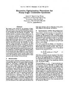
Figure 2: Convergent bounds for test problem Bex2 1 1

column holds the objective value computed by GloptiPoly. The following six columns include the results computed by our method. In particular, p∗ω corresponds to the optimal objective value and in this column the sequence of lower bounds computed is reported. The upper bound is equal to the lower bound within accuracy ǫ = 10−6 , hence its value is implied. The subsequent column reports the maximun relaxation order needed in the subproblems and the relaxed master problems, i.e. ω in and ω out , respectively, until global optimality is reached. The number of iterations, the average cpu time per iteration, and the values of the metrics (44) are stated in the last four columns. Observe that when a rational iteration number is reported, it means that our procedure terminated at Step 4.1, while an integer iteration number means that our procedure terminated at Step 3. Note also that the times reported aim only at giving an indicative idea of the average time spent per iteration by our procedure. Due to the testing status of our code several redundant readings and writings increase the actual time spent.

18

Partitioning Procedure for POPs

GloptiPoly

19

Problem

n

m

p∗

ω

p∗ ω,bmrk

p∗ ω

(ωin , ωout )

iters

cputime/iter

ǫp∗

ǫ x∗

Wol3 5

4

3

−7

3

−7

{−9, . . . , −7}

(2, 1)

2

0.67

3.32e − 09

5.37e − 09

Wol4 2

4

6

−13

2

−13

{−13, . . . , −13}

(1, 1)

1 21

1.12

8.37e − 10

2.65e − 09

Bex2 1 1

5

1

−17

3

−17

{−454.955, . . . , −17}

(3, 4)

3

4.71

3.76e − 09

7.49e − 09

Bex2 1 2

6

2

−213

2

−213

{−217, . . . , −213}

(2, 2)

2

2.89

7.29e − 10

3.46e − 08

Bex2 1 4

6

5

−11

2

−11

{−11, . . . , −11}

(2, 1)

1

3.68

7.13e − 08

8.02e − 10

Bex2 1 5

10

11

−268.0146

2

−268.015

{−284.236, . . . , −268.015}

(2, 2)

3

10.70

3.26e − 07

5.86e − 06

Bex3 1 2

5

6

−30665.5

2

−30665.5

{−39492.7, . . . , −30665.5}

(2, 1)

4

2.54

8.90e − 10

3.25e − 09

Bex9 1 1

13

12

−13

2

−13

{−45868.1, . . . , −13}

(1, 1)

3

2.83

7.62e − 10

5.93e − 03

Bex9 1 2

10

9

−16

3

−

{−16.5556, . . . , −16}

(1, 1)

2

0.88

−

−

Bex9 1 4

10

9

−37

3

−

{−106.968, . . . , −37}

(1, 2)

2

1.38

−

−

Bex9 2 4

8

7

0.5

2

0.499889

{0.24, . . . , 0.49}

(2, 1)

6

21.04

9.31e − 03

4.02e − 02

Bex9 2 5

8

7

5.0

2

5.00004

{−46.1465, . . . , 5}

(1, 2)

6

2.31

7.62e − 06

3.55e − 04

Bex9 2 8

6

5

1.5

2

1.5

{1.185, . . . , 1.5}

(2, 1)

3

2.23

4.95e − 09

3.72e − 09

meanvar

8

2

5.2434

2

5.2434

{5.2434, . . . , 5.2434}

(1, 1)

1

0.00

1.50e − 09

1.05e − 05

Bst bpaf1a

10

10

−

2

−45.3797

{−45.3797, . . . , −45.3797}

(1, 1)

1 21

2.36

3.47e − 09

7.38e − 08

Bst bpaf1b

10

10

−

2

−42.9626

{−42.9626, . . . , −42.9626}

(1, 1)

1 21

2.38

8.77e − 09

6.60e − 08

Bst e05

5

3

−

3

7049.25

{2739.29, . . . , 7049.23}

(1, 1)

24 21

1.89

3.34e − 06

9.25e − 04

Bst e07

10

7

−

2

−1809.18

{−2283.98, . . . , −1809.2}

(1, 3)

2

1.81

9.34e − 06

8.77e − 03

Bst jcbpaf2

10

13

−

2

−794.856

{−1259.28, . . . , −794.944}

(1, 1)

20

3.35

1.11e − 04

1.86e − 02

st e21

6

6

−

2

−14.1

{−16.7, . . . , −14.1}

(1, 1)

2 12

0.37

3.80e − 10

5.28e − 10

Continued on next page

Partitioning Procedure for POPs

GloptiPoly Problem

n

m

p∗

ω

p∗ ω,bmrk

p∗ ω

(ωin , ωout )

iters

cputime/iter

ǫp∗

ǫ x∗

st glmp kk90

5

7

−

2

3

{−146.315, . . . , 3}

(2, 1)

2

1.66

7.23e − 11

1.95e − 09

Table 1: Partitioning Procedure for POPs and GloptiPoly on test problems

20

As can be seen, in all cases our procedure and GloptiPoly gave equally satisfactory results. In two cases, i.e. Problems Bex9 1 2 and Bex9 1 4, our procedure outperformed GloptiPoly. However, the POPs we handled with our procedure are still small to medium size. Further improvements are essential to be able to tackle larger problems. For instance, we can customize the partitioning of variables according to the sparse structure of the problem, if any [28, 29, 30]. The sparsity pattern of the POP would help us partition the set of variables, not randomly, but based on its sparsity structure, in more than one subsets. This controlled partitioning of polynomial variables would produce more than one smaller-size POP subproblems at Step 4, hence easier to tackle. On the other hand, the numerical results reported in the following section show a considerable improvement in terms of problem size.

5

Application to Portfolio Decisions with Higher Order Moments

In this section, we consider the problem of selecting an optimal investment portfolio that consists of holdings in a number of assets. According to the classical mean-variance approach devised by [31] the investors goal is to maximize the expected return of the portfolio (first moment or mean) and minimize its risk (second central moment or variance). However, this model is based on the assumption that asset returns are normally distributed. As empirical evidence suggests [32], normality may not be the case in reality. On the contrary, asset return distributions are generally characterized by asymmetries and/or fat tails. In order to relax this assumption, we incorporate skewness (third central moment) and kurtosis (fourth central moment) in the optimal portfolio selection. In our model the investor’s goal is to maximize the expected return and the skewness of the portfolio, and minimize the variance and the kurtosis of the portfolio, subject to satisfying the budget constraint and excluding short sales. The consideration of higher moments in portfolio selection dates back in early sixties [33]. The interested reader is referred to [34, 35, 36] and the many references therein for recent advances.

5.1

Problem Formulation

Notation: In this section, Rit denotes the return on asset i at time t and N the total number of returns on asset i; Ri expresses the average return on asset i. Let µi be the expected return (mean) of Ri and σij be the covariance of Ri and Rj . Similarly, let sijk be the coskewness of

21

Moment

Symbol

Expected return (Mean) of asset i

µi

Variance of asset i

σii

Skewness of asset i

siii

Kurtosis of asset i

kiiii

Covariance of assets i and j

σij

Coskewness of assets i, j and k

sijk

Cokurtosis of assets i, j, k and l

kijkl

Table 2: Asset Statistics (Moments): Symbols

Moment

Definition

µi

E[Ri ]

σii

E[(Ri − µi )2 ]

siii kiiii

Formula N 1 X Rit N t=1 N X 1

(Rit − µi )2

E[(Ri − µi )3 ]

N −1 N 1 X

(Rit − µi )3

E[(Ri − µi )4 ]

t=1 N X

(Rit − µi )4

N 1 N

σij

E[(Ri − µi )(Rj − µj )]

sijk

E[(Ri − µi )(Rj − µj )(Rk − µk )]

kijkl

E[(Ri − µi )(Rj − µj )(Rk − µk )(Rl − µl )]

t=1

t=1

N X 1 (Rit − µi )(Rjt − µj ) N − 1 t=1 N 1 X (Rit − µi )(Rjt − µj )(Rkt − µk ) N t=1 N 1 X (Rit − µi )(Rjt − µj )(Rkt − µk )(Rlt − µl ) N t=1

Table 3: Asset Statistics (Moments): Definitions and Formulae

Ri , Rj and Rk and kijkl the cokurtosis of Ri , Rj , Rk and Rl 7 . These asset statistics and their formulae are summarized in Tables 2 and 3, respectively. We consider a portfolio of n risky assets held over a single period. The profit R on the portfolio as Pn whole is R = i=1 xi Ri , where xi is the proportion of the portfolio invested on asset i. Observe that the Ri ’s and consequently R, are random variables. Hence, the return R of the portfolio is a

weighted sum of random variables, where the investor seeks to find the weights so as to maximize his profit with a low risk. Thus, the portfolio weights x1 , . . . , xn are the objective variables in the optimization problem that arises. In our analysis, short sales are excluded, so we have that xi ≥ 0 for all i. Also, because xi ’s are percentages and not the actual amount invested on each asset, we Pn have that i=1 xi = 1 to represent the budget constraint. These two types of constraints form a 7 Observe

that σii , siii , kiiii are the variance, skewness and kurtosis of Ri , respectively.

22

polyhedral set of feasible portfolios, n

X = {x ∈ IR |

n X

xi = 1, x ≥ 0}.

(45)

i=1

Then, for fixed probability beliefs (µi , σij , sijk , kijkl ), the problem of choosing the optimal portfolio based on the first four moments of the portfolio return is: max α x∈X

n X i=1

µi xi − β

n X

σij xi xj + γ

i,j=1

n X

i,j,k=1

sijk xi xj xk − δ

n X

kijkl xi xj xk xl .

(46)

i,j,k,l=1

The scalars α to δ are the investor’s preferences to the four moments and they sum up to one, i.e. α + β + γ + δ = 1. The objective function in formulation (46) is a real-valued polynomial of degree four, the objective vector is x ∈ IRn and the feasible set is a (n − 1)-simplex; hence, the resulting problems are POPs of total degree four.

23

Mean

Variance

Skewness

Kurtosis

Mean

Variance

Skewness

Kurtosis

24

Asset 1

−1.66e − 03

3.47e − 03

−3.52e − 04

1.93e − 04

Asset 11

2.03e − 03

4.34e − 03

2.04e − 04

4.18e − 04

Asset 2

1.42e − 03

1.38e − 03

1.25 − 05

1.35e − 05

Asset 12

6.18e − 03

2.85e − 03

3.85e − 05

3.29e − 05

Asset 3

6.44e − 04

5.28e − 03

−4.17e − 04

3.17e − 04

Asset 13

4.44e − 04

1.74e − 03

1.07e − 05

1.88e − 05

Asset 4

−2.39e − 04

3.12e − 03

−5.90e − 04

3.44e − 04

Asset 14

1.08e − 02

1.05e − 02

2.47e − 03

2.06e − 03

Asset 5

3.22e − 03

1.76e − 02

3.89e − 03

4.88e − 03

Asset 15

1.49e − 03

1.90e − 03

−2.80e − 04

1.52e − 04

Asset 6

9.63e − 04

1.78e − 03

−1.11e − 04

5.88e − 05

Asset 16

2.91e − 04

5.39e − 03

−5.48e − 04

4.83e − 04

Asset 7

8.15e − 04

9.83e − 03

5.30e − 05

5.33e − 04

Asset 17

−8.31e − 04

3.03e − 03

−8.57e − 04

5.25e − 04

Asset 8

2.19e − 03

5.07e − 03

−1.16e − 04

1.53e − 04

Asset 18

1.78e − 03

3.47e − 03

−6.04e − 04

3.23e − 04

Asset 9

2.54e − 03

5.40e − 03

−2.85e − 05

1.29e − 04

Asset 19

1.31e − 03

4.61e − 03

−9.43e − 05

1.95e − 04

Asset 10

2.48e − 03

4.54e − 03

−2.52e − 05

1.80e − 04

Asset 20

8.02e − 04

9.00e − 04

−3.47e − 06

5.57e − 06

Table 4: The values of the four moments of each component of our portfolio

5.2

Numerical Results

For randomly generated investor’s preferences (α, β, γ, δ), we applied our algorithm to the resulting portfolio selection problems formulated as in (46). The portfolio included a collection of assets from the S&P 500 US index. We obtained weekly historical prices covering a period of ten years from uk.finance.yahoo.com. In Table 4, the computed probability beliefs (moments) of each asset are presented8 . Table 5 contains the optimal portfolios for each investor preference (α, β, γ)9 after we applied our procedure to problem (46) using the data of Table 4. In particular, the investor preferences, the optimal vector x of portfolio weights10 (multiplied by ten), and the optimal values of the four portfolio moments are reported in the first six columns of the table. The last column holds the number of iterations performed by our algorithm such that a 10−6 accuracy between the lower and upper bounds computed is achieved. As Table 5 reveals, the optimization of the first four moments of a portfolio consisting of twenty assets can be solved efficiently by our procedure in six iterations on average. The results of Table 5 reinforce our belief that decomposition may play an important role in large-scale polynomial programming.

8 The

comoments, such as covariance, coskewness and cokurtosis, have not been included in the table. value of δ is implied since the four parameters sum up to one, i.e. α + β + γ + δ = 1. 10 Note that all reported portfolio weights add up to one, but due to rounding may not appear to do so. 9 The

25

26

(α, β, γ)

10 ∗ x

P. Mean

P. Var

P. Skew

P. Kurt

Iter

(1.00, 0.00, 0.00)

(0.0, 0.0, 0.0, 0.0, 10.0, 0.0, 0.0, 0.0, 0.0, 0.0, 0.0, 0.0, 0.0, 0.0, 0.0, 0.0, 0.0, 0.0, 0.0, 0.0)

3.22e − 03

1.76e − 02

3.89e − 03

4.88e − 03

1

(0.74, 0.13, 0.01)

(0.0, 0.0, 0.0, 0.0, 1.1, 0.0, 0.0, 0.0, 0.0, 0.2, 0.0, 0.0, 0.0, 8.7, 0.0, 0.0, 0.0, 0.0, 0.0, 0.0)

9.47e − 03

8.30e − 03

1.60e − 03

1.18e − 03

3

(0.14, 0.20, 0.20)

(0.0, 5.2, 0.0, 0.0, 0.6, 1.1, 0.0, 0.8, 0.9, 1.4, 0.0, 0.0, 0.0, 0.0, 0.0, 0.0, 0.0, 0.0, 0.0, 0.0)

1.79e − 03

8.07e − 04

−1.73e − 06

1.81e − 06

5

(0.34, 0.29, 0.34)

(0.0, 0.8, 0.0, 0.0, 0.3, 0.0, 0.0, 0.4, 0.3, 1.3, 0.0, 3.6, 0.0, 3.3, 0.0, 0.0, 0.0, 0.0, 0.0, 0.0)

6.28e − 03

1.73e − 03

7.72e − 05

2.43e − 05

7

(0.05, 0.77, 0.08)

(0.0, 1.2, 0.1, 0.0, 0.1, 0.3, 0.0, 0.0, 0.0, 0.0, 0.3, 1.0, 1.7, 0.1, 0.6, 0.0, 0.0, 0.0, 0.0, 4.5)

1.60e − 03

4.25e − 04

−2.65e − 06

5.73e − 07

10

(0.31, 0.18, 0.21)

(0.0, 1.2, 0.0, 0.0, 0.6, 0.0, 0.0, 0.0, 0.0, 1.0, 0.0, 2.8, 0.0, 4.4, 0.0, 0.0, 0.0, 0.0, 0.0, 0.0)

7.12e − 03

2.65e − 03

2.01e − 04

8.03e − 05

6

(0.28, 0.38, 0.17)

(0.0, 2.8, 0.0, 0.0, 0.3, 0.0, 0.0, 0.1, 0.0, 0.7, 0.0, 3.9, 0.0, 2.3, 0.0, 0.0, 0.0, 0.0, 0.0, 0.0)

5.52e − 03

1.31e − 03

2.40e − 05

7.34e − 06

6

(0.03, 0.70, 0.15)

(0.0, 1.8, 0.3, 0.2, 0.2, 1.2, 0.0, 0.0, 0.0, 0.0, 0.1, 0.3, 1.3, 0.0, 0.0, 0.0, 0.0, 0.0, 0.0, 4.6)

1.07e − 03

4.17e − 04

−2.93e − 06

6.70e − 07

6

(0.17, 0.24, 0.35)

(0.0, 5.3, 0.0, 0.0, 0.6, 1.0, 0.0, 0.8, 1.0, 1.4, 0.0, 0.0, 0.0, 0.0, 0.0, 0.0, 0.0, 0.0, 0.0, 0.0)

1.80e − 03

8.15e − 04

−1.63e − 06

1.83e − 06

5

(0.08, 0.24, 0.13)

(0.0, 5.1, 0.3, 0.0, 0.4, 1.9, 0.0, 0.6, 0.7, 1.0, 0.0, 0.0, 0.0, 0.0, 0.0, 0.0, 0.0, 0.0, 0.0, 0.0)

1.60e − 03

7.22e − 04

−3.02e − 06

1.85e − 06

5

(0.10, 0.01, 0.51)

(0.0, 0.0, 0.0, 0.0, 7.8, 0.0, 0.0, 0.0, 1.2, 1.1, 0.0, 0.0, 0.0, 0.0, 0.0, 0.0, 0.0, 0.0, 0.0, 0.0)

3.06e − 03

1.11e − 02

1.84e − 03

1.80e − 03

6

(0.09, 0.20, 0.07)

(0.0, 5.2, 0.2, 0.0, 0.5, 1.8, 0.0, 0.6, 0.7, 1.2, 0.0, 0.0, 0.0, 0.0, 0.0, 0.0, 0.0, 0.0, 0.0, 0.0)

1.65e − 03

7.38e − 04

−2.69e − 06

1.81e − 06

5

(0.22, 0.02, 0.63)

(0.0, 0.0, 0.0, 0.0, 10.0, 0.0, 0.0, 0.0, 0.0, 0.0, 0.0, 0.0, 0.0, 0.0, 0.0, 0.0, 0.0, 0.0, 0.0, 0.0)

3.22e − 03

1.76e − 02

3.89e − 03

4.88e − 03

5

Table 5: Portfolio weights and portfolio moments after optimization

6

Conclusions and Future Plans

In this paper it is intended to show that the Benders decomposition can be extended to polynomial optimization problems using Stengle’s Positivstellensatz in place of the Farkas lemma and Putinar’s Positivstellensatz in place of the convex duality theorem. The lack of convexity in our problems and the polynomial functions involved necessitates the use of the sum-of-squares representation. This representation yields polynomial functions instead of constant multipliers for the generation of feasibility and optimality constraints. The theoretical results in this work are in line with those presented in [7], where nonconvex problems are also tackled and the use of duality theory for general programs produces functions in place of constant multipliers. However, the sum-ofsquares representation only ensures asymptotic convergence of our procedure. Finite convergence remains to be investigated in the future. From the computational perspective, the numerical results presented appear to be satisfactory. These are even more promising in the case of the application to portfolio selection with higher order moments. To improve the efficiency of our procedure, for sparse POPs, we intend to replace the optimality and feasibility constraints introduced here by their sparse analog based on the results introduced in [28, 29]. Such an amendment is expected to simplify the optimality/feasibility constraints formulation. Hence, this would result in a smallersize and easier to tackle master problem. In addition, the sparsity of the POP, if exists, should enable us not to partition the set of variables randomly, but based on its sparsity structure, and derive smaller-size subproblems.

7

Acknowledgments

The authors would like to thank the two anonymous referees for their stimulating remarks and helpful comments.

References [1] J. F. Benders. Partitioning procedures for solving mixed-variables programming problems. Computational Management Science, 2(1):3–19, 2005. Reprinted from Numerische Mathematik 4 (1962), 238–252. [2] A. Prestel and C. N. Delzell. Positive polynomials. Springer Monographs in Mathematics. Springer-Verlag, Berlin, 2001. From Hilbert’s 17th problem to real algebra.

27

[3] J. B. Lasserre. Global optimization with polynomials and the problem of moments. SIAM Journal on Optimization, 11(3):796–817, 2000/01. [4] P. A. Parrilo. Semidefinite programming relaxations for semialgebraic problems. Mathematical Programming, 96(2, Ser. B):293–320, 2003. Algebraic and geometric methods in discrete optimization. [5] A. Ben-Tal and A. Nemirovski. Lectures on modern convex optimization. MPS/SIAM Series on Optimization. Society for Industrial and Applied Mathematics (SIAM), Philadelphia, PA, 2001. Analysis, algorithms, and engineering applications. [6] A. M. Geoffrion. Generalized Benders decomposition. Journal of Optimization Theory and Applications, 10:237–260, 1972. [7] L. A. Wolsey. A resource decomposition algorithm for general mathematical programs. Mathematical Programming Study, (14):244–257, 1981. Mathematical programming at Oberwolfach (Proc. Conf., Math. Forschungsinstitut, Oberwolfach, 1979). [8] C. A. Floudas and V. Visweswaran. A global optimization algorithm (GOP) for certain classes of nonconvex NLPs: I. theory. Computers & chemical engineering, 14(12):1397–1417, 1990. [9] V. Visweswaran and C. A. Floudas. A global optimization algorithm (GOP) for certain classes of nonconvex NLPs: II. application of theory and test problems. Computers & chemical engineering, 14(12):1419–1434, 1990. [10] V. Visweswaran and C. A. Floudas. Unconstrained and constrained global optimization of polynomial functions in one variable. Journal of Global Optimization, 2(1):73–99, 1992. Conference on Computational Methods in Global Optimization, I (Princeton, NJ, 1991). [11] M. Laurent. Sums of squares, moment matrices and optimization over polynomials. In Emerging applications of algebraic geometry, volume 149 of IMA Volumes in Mathematics and its Applications, pages 157–270. Springer, New York, 2009. [12] G. Stengle. A nullstellensatz and a positivstellensatz in semialgebraic geometry. Mathematische Annalen, 207:87–97, 1974. [13] D. Cox, J. Little, and D. O’Shea. Ideals, varieties, and algorithms. Undergraduate Texts in Mathematics. Springer-Verlag, New York, 1992. An introduction to computational algebraic geometry and commutative algebra. [14] K. Schm¨ udgen. The K-moment problem for compact semi-algebraic sets. Mathematische Annalen, 289(2):203–206, 1991.

28

[15] M. Schweighofer. Optimization of polynomials on compact semialgebraic sets. SIAM Journal on Optimization, 15(3):805–825, 2005. [16] M. Putinar. Positive polynomials on compact semi-algebraic sets. Indiana University Mathematics Journal, 42(3):969–984, 1993. [17] J. Nie and M. Schweighofer. On the complexity of Putinar’s Positivstellensatz. Journal of Complexity, 23(1):135–150, 2007. [18] A. M. Geoffrion. Elements of large-scale mathematical programming. I. Concepts. Management Science. Journal of the Institute of Management Science. Application and Theory Series, 16:652–675, 1969/70. [19] P. A. Parrilo. Algebraic techniques and semidefinite optimization. MIT 6.972 Lecture Notes, 2006. [20] R. Meyer. The validity of a family of optimization methods. SIAM Journal on Control and Optimization, 8:41–54, 1970. [21] J. Tind and L. A. Wolsey. An elementary survey of general duality theory in mathematical programming. Mathematical Programming, 21(3):241–261, 1981. [22] H. Tuy. Convex analysis and global optimization, volume 22 of Nonconvex Optimization and its Applications. Kluwer Academic Publishers, Dordrecht, 1998. [23] W. W. Hogan. Point-to-set maps in mathematical programming. SIAM Review, 15:591–603, 1973. [24] D. Henrion and J. B. Lasserre. GloptiPoly: global optimization over polynomials with Matlab and SeDuMi. ACM Transactions on Mathematical Software, 29(2):165–194, 2003. [25] J. F. Sturm. Using SeDuMi 1.02, a MATLAB toolbox for optimization over symmetric cones. Optimization Methods and Software, 11/12(1-4):625–653, 1999. [26] C. A. Floudas and P. M. Pardalos. A collection of test problems for constrained global optimization algorithms, volume 455 of Lecture Notes in Computer Science. Springer-Verlag, Berlin, 1990. [27] GLOBAL Lib, 2008. www.gamsworld.org/global/globallib/globalstat.htm. [28] J. B. Lasserre. Convergent SDP-Relaxations in Polynomial Optimization with Sparsity. SIAM Journal on Optimization, 17(3):822–843, 2006.

29

[29] H. Waki, S. Kim, M. Kojima, and M. Muramatsu. Sums of squares and semidefinite program relaxations for polynomial optimization problems with structured sparsity. SIAM Journal on Optimization, 17(1):218–242 (electronic), 2006. [30] P. M. Kleniati, P. Parpas, and B. Rustem. Decomposition-Based Method for Sparse Semidefinite Relaxations of Polynomial Optimization Problems. To appear in Journal of Optimization, Theory and Applications 145/2, 2010. [31] H. Markowitz. Portfolio selection. Journal of Finance, 7:77–91, 1952. [32] P. M. Kleniati. Portfolio optimization with skewness. Master’s thesis, Department of Computing, Imperial College, London, UK, 2004. [33] B. Mandelbrot. The variation of certain speculative prices. Journal of Business, 36:394, 1963. [34] E. Jondeau and M. Rockinger. Optimal Portfolio Allocation under Higher Moments. European Financial Management, 12(1):29–55, 2006. [35] P. M. Kleniati and B. Rustem. Portfolio decisions with higher order moments. Working Paper, 2009. [36] D. Maringer and P. Parpas. Global optimization of higher order moments in portfolio selection. Journal of Global Optimization, 43(2-3):219–230, 2009.

30