Clinical Chemistry 57:3 475–481 (2011)
Informatics and Statistics
Partitioning Reference Intervals by Use of Genetic Information Brian H. Shirts,1* Andrew R. Wilson,2 and Brian R. Jackson1,2
BACKGROUND: Reference intervals that incorporate genetic information could reduce the misidentification of unusual test results caused by non– diseaseassociated genetic variation and increase the detection of results indicating underlying pathology. Subdividing reference groups by genetic effects, however, may lead to increased uncertainty around reference interval endpoints (because of the smaller subgroup sample sizes), thus offsetting any benefits. METHODS:
We evaluated CLSI guidelines to develop a method appropriate for partitioning reference intervals on the basis of genetic variants with dominant or recessive effects. This method uses information available before reference samples are recruited, thus allowing a preliminary decision regarding partitioning to be made before sampling. We used this method to evaluate the example of Gilbert syndrome.
RESULTS:
The decision point for partitioning occurs when the percentage of total variance attributable to a dominant or recessive genetic polymorphism exceeds 4%. Similarly, partitioning decision curves are presented based on difference in means between 2 subgroups, sample SD, and subgroup or allele frequency. Laboratory-specific partitioned reference intervals for Gilbert syndrome appear to be statistically warranted for white and African-American populations, but not for Asian populations.
CONCLUSIONS: We present a simple method to evaluate whether partitioning based on dominant or recessive genetic effects is statistically justified. Important limitations remain that, in many situations, will preclude integration of genetic, laboratory, and clinical information. As society moves toward personalized medicine, additional research is needed on how to evaluate patient normality while accounting for additive genetic, multigenic, and other multifactorial effects.
© 2010 American Association for Clinical Chemistry
1
Department of Pathology, University of Utah School of Medicine, Salt Lake City, UT; 2 ARUP Institute for Clinical and Experimental Pathology, Salt Lake City, UT. * Address correspondence to this author at: University of Utah Health Sciences Center, Department of Pathology, 15 North Medical Dr., Suite 1100, Salt Lake City, UT 84112. E-mail
[email protected].
The most common statistical tool used by clinicians to evaluate between-patient variation is the populationbased reference value. Ideally, reference values are determined by individual laboratories measuring the analyte levels in a group of reference individuals who are healthy and representative of the population the laboratory serves (1 ). Reference values are often partitioned on the basis of demographic variables that are known to influence analyte levels, such as sex and age. Partitioning can reduce variance and improve the predictive utility of the reference intervals. Similarly, reducing variance by partitioning based on genetic differences could potentially reduce between-person variation and improve the quality of laboratory information in clinical diagnosis. The current cost of clinical genotyping is generally prohibitive; however, the cost of genotyping is rapidly dropping. As whole-genome data becomes clinically available and more associations between genetic polymorphisms and laboratory test results are discovered, clinical chemists may begin to search for ways of integrating genetic information with laboratory information to improve the performance characteristics of laboratory tests. Integrating genetic and laboratory information, where appropriate, would increase the accuracy of reference intervals by eliminating extreme results related to genetic variation, thereby increasing the percentage of extreme results that reflect underlying pathology. Unfortunately, if the difference between groups is small, the benefit of subdividing may be offset by the increased uncertainty around endpoint estimates caused by the decrease in sample size. Although more personalized medicine has become a goal of many public health and research organizations, generating and partitioning reference intervals is a labor- and costintensive exercise. Before going to the effort of collecting extra data for partitioning based on genetic information, laboratory directors will wish to know if including additional variables would improve the performance characteristics of reference intervals.
A portion of this material was presented in abstract and poster form at the annual meeting of the Association for Molecular Pathology, San Jose, California, November 2010. Received July 23, 2010; accepted November 15, 2010. Previously published online at DOI: 10.1373/clinchem.2010.154005
475
Our goal was to investigate issues that may arise if laboratories wish to use genetic information to partition reference intervals and to provide a framework that, for simple situations, allows an estimate to be made about the utility of partitioning before beginning sample recruitment for reference studies. We used standard guidelines for partitioning reference intervals to determine if these suggest a method to determine when it might make sense for a clinical laboratory to generate genotype-specific reference intervals. We evaluate a statistical framework for use of a single dominant or recessive genetic variant to partition a sample into 2 groups using standard information likely to be reported in the scientific literature or available to a laboratory director, such as the difference in mean level of the analyte, the SD of the analyte, and the percentage of population variance attributed to a genetic variant. Although developed for genetic factors, this method could also be used to evaluate a priori decisions on partitioning based on other factors, such as race (which has genetic components), smoking status, or other specific environmental exposures. Our method highlights some of the limitations of standard statistical practices for evaluating the utility of integrating genetic and clinical tests, which we will discuss. We discuss the example of Gilbert syndrome to illustrate the partitioning decision process.
gested sizes for partitioned samples are often much larger than those for unpartitioned samples (1 ). If estimates of expected difference between subsample means and subsample SDs are available, the Harris and Boyd method makes it possible to evaluate if partitioning is warranted before recruiting volunteers. Briefly, CLSI guidelines strongly recommend direct sampling, where reference individuals represent the population a laboratory serves based on specific, well-defined criteria for appropriate health (1 ). For partitioning, if subsample SDs are similar, a z-statistic is calculated for the difference between distribution means: Z⫽
兩x 1 ⫺ x 2 兩
冑冋冉 冊 冉 冊册 22 12 ⫹ n1 n2
,
(1)
where x 1 and x 2 are the subpopulation means, n1 and n2 are the number of individuals in each subgroup, and 12 and 22 are the subpopulation variances (3 ). A z-statistic that is above a given cutoff suggests that the groups should be partitioned. The suggested cutoff for z-statistics formulated by Harris and Boyd (2 ) and reiterated in more general form by CLSI guidelines (1 ) is:
Statistical Background on the Decision to Partition
冑
Accepted methods for determining reference intervals are outlined in CLSI documents (1 ), which are based on the work of Harris and Boyd (2 ). To understand the rationale behind the Harris and Boyd approach, consider a situation in which a laboratory partitions a reference interval for a particular analyte by patient sex. To do this, the laboratory might recruit 120 men and 120 women and then determine the central 95% interval for each group. But now consider the situation of an analyte that has only a very small difference between men and women. In such a case, combining all the volunteers into a larger group of 240 individuals would produce a more statistically defensible central 95% such that it might end up being more accurate overall than the separate male and female reference intervals. It may even be the case that fewer than 240 reference individuals will produce a common reference interval that is more accurate than the partitioned intervals. Thus, partitioning is useful only when underlying factors, such as sex or genotype, are responsible for a difference in analyte levels that is large enough to generate more precise intervals given the reference sample size. It can be important to know before recruiting volunteers whether partitioning will likely be useful, because this can influence the size of the desired sample, as sug-
This z-statistic cutoff was set such that partitioning will be recommended when the proportions of individuals above or below the expected lower and upper (2.5% or 97.5%) cutoffs for subpopulations will be substantially different from those expected by clinicians (e.g., ⬎4% rather than 2.5%). Although the method was developed to partition reference ranges for which the subgroups are approximately equal in size and follow a gaussian distribution, others have suggested that the method is reasonable for samples of unequal size as long as the SDs are similar, and that the z-statistic may also be appropriate for nongaussian distributions when there are at least 60 individuals in each subgroup (1, 3, 4 ). Where there are extreme deviations from normality or large differences in subgroup prevalence, other methods—such as those proposed by Lahti and colleagues (4, 5 )—may be more appropriate. Inconsistencies between the Harris and Boyd method and other partitioning methods have been noted, particularly for large reference samples, in which the Harris and Boyd method may fail to partition even when there are substantial differences between reference populations (6 ). On the other hand, we have found that Lahti’s methods often inappropriately stratify groups randomly selected from the same population if the reference sample is ⬍1000 individuals (data not shown).
476 Clinical Chemistry 57:3 (2011)
Z* ⫽ 3
n1 ⫹ n2 . 240
(2)
Partitioning Reference Intervals by Use of Genetic Data
Partitioning Cutoffs in Relation to Proportion of Variance For 2 subgroups with equal variance, the total population variance is a function of the subgroup variance, means of the subgroups, and the relative frequencies of the populations:
t2 ⫽ g2 ⫹ 共a 1 a 2 兲共 x 1 ⫺ x 2 兲 2 ,
(3)
where t is the total variance, g ⫽ 1 ⫽ 2 is variance of the subgroups, x 1 and x 2 are subgroup means, and a1 and a2 are the relative proportions of the total group made up by each subgroup such that n1 ⫽ a1N, n2 ⫽ n2N, and a1 ⫹ a2 ⫽ 1, where N is the total sample size. If the variance attributable to the factor that distinguishes a1 and a2 is represented by , then t2 ⫽ g2 ⫹ and the proportion of the total variance attributable to the factor is /t2. In this situation, the numerator of the z-statistic (Eq. 1) can be expressed in terms of : 2
2
Z⫽
2
冑
a 1a 2
g
冑冋冉 冊 冉 冊册 1 1 ⫹ a 1N a 2N
2
.
(4)
If z is set to be equal to Harris and Boyd’s recommended cutoff for z* (Eq. 2), then cutoff values can be expressed as a function of proportion of total variance attributable to a polymorphism () and the sample proportions a1 and a2:
3
冑
共a 1 N兲 ⫹ 共a 2 N兲 ⫽ 240
冑
a 1a 2
g
冑冋冉 冊 冉 冊册 1 1 ⫹ a 1N a 2N
,
(5) which simplifies (see Supplemental Appendix I, which accompanies the online version of this article at www.clinchem.org/content/vol57/issue3, for a more detailed derivation): 3 ⫽ 0.039. 2 ⫽ t 77
(6)
Thus, a proportion of the total variance of 4% or greater would justify partitioning into 2 groups if subsamples have equal SDs. This partitioning cutoff does not change for large or small relative sample proportions because the calculation of variance already accounts for the influence of sample proportion. We assume that the subsample proportions in the reference sample are approximately equal to the sub-
sample proportions in the population, which should be a reasonable assumption if the reference sample has been recruited randomly or been selected to appropriately represent the population the laboratory serves and if the sample is of reasonable size. If the sample proportion (a1), difference between subpopulation means (x 1 ⫺ x 2), and total sample variance (t2) or SD (t) are known, it is straightforward to calculate a similar cutoff. This expression of the cutoff, while more complicated, may be useful for a priori partitioning decisions, as these values are often more easily obtained than the proportion of total variance attributed to a partitioning factor. As sample proportion and ratio of difference in mean between subsamples to total sample SD (x 1 ⫺ x 2)/t, changes, so does the proportion of total variance attributable to the partitioning factor: 共 x 1 ⫺ x 2 兲 ⫽ t
冑
3 . 77a 1 a 2
(7)
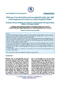
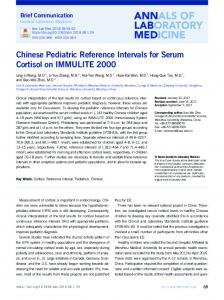
This relationship is plotted in Fig. 1. If a population was equally subdivided, a1 ⫽ 0.5, then a difference in means 共x 1 ⫺ x 2兲 greater than approximately 40% of the SD: t ⱖ 0.4, would justify partitioning. If the difference between the means of the subpopulations was equal to 共x 1 ⫺ x 2兲 the SD: ⫽ 1, partitioning would be justified if t the frequency of the smaller population were 4% or more, a1 ⱖ 0.04 (see Fig. 1). Partitioning by a Genetic Variant with Dominant or Recessive Effects by Use of Minor Allele Frequency Partitioning where a genetic polymorphism has dominant or recessive effects with attributable variance of 4% or greater would be practical, as illustrated above. However, genetic studies often report minor allele frequencies (MAFs) rather than population proportions. If MAF is reported with difference in mean between 2 alleles and the total sample variance is available, then one can evaluate Eq. 7 by representing population proportions in terms of genetic alleles. In standard genetic nomenclature, MAF is q, and the frequency of the common or major allele is p, such that p ⫹ q ⫽1. It is often the case that subpopulations are in Hardy–Weinberg equilibrium represented by the equation: p2 ⫹ 2pq ⫹ q2 ⫽ 1. Most genetic polymorphisms that influence quantitatively measured analyte levels do not influence variance of subpopulations, so the assumption that subgroups defined by genetic polymorphisms have equal variance is almost always true. A genetic variant with recessive effects divides the population into 2 subpopulations with proportions Clinical Chemistry 57:3 (2011) 477
Fig. 1. Partitioning cutoff as a function of the difference in mean to SD ratio, (x 1 ⴚ x 2)/t, and the sample proportion, a1. When (x 1 ⫺ x 2)/t and a1 fall in the area above the curve, partitioning using a sample recruited randomly from the population will be reasonable, and when (x 1 ⫺ x 2)/t and a1 fall in the area below the lowest point on the curve, no benefit to partitioning is likely. When these parameters fall below the line but above 0.4 (the lowest point on the curve), there may be benefit to partitioning, but that population-based recruitment would result in reference intervals for that subsample that are unlikely to produce a more statistically defensible central 95% for this group than the cutoffs defined by the larger sample.
a1 ⫽ p2 and a2 ⫽ 2pq ⫹ q2, which can be substituted into Eq. 7: 共 x 1 ⫺ x 2 兲 ⫽ t
冑
3 . 77共 p 2 兲共2pq ⫹ q 2 兲
(8)
The equation for dominant effects is generated by simply reversing proportions of a1 and a2: 共 x 1 ⫺ x 2 兲 ⫽ t
冑
3 . 77共 p 2 ⫹ 2pq兲共q 2 兲
(9)
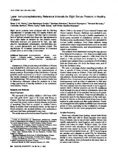
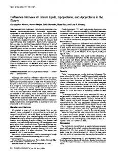
These equations can be used to generate the decision curves presented in Fig. 2, which are mirror images of each other. As above, these equations are based on the assumption that the subsample proportions of the reference sample— genetic allele frequencies, in this case—are approximately equal to the frequencies in the reference population. Discussion PRACTICAL INTERPRETATION OF PARTITIONING CUTOFFS
Laboratories that conduct reference value studies ideally define selection criteria and potential partitioning 478 Clinical Chemistry 57:3 (2011)
parameters before recruiting reference individuals (1 ). Our analysis suggests 3 situations that laboratories may encounter when considering partitioning by use of a single dominant or recessive genetic trait: 1. The genetic effect is not large enough to justify partitioning; if the difference between subpopulation means is ⬍40% of the subsample SDs, the genetic effect would not justify partitioning (the area below the lowest point of either curve in Fig. 2). 2. The genetic effect is large enough to justify partitioning and the genetic polymorphism is common enough to justify population-based recruitment, if ⱖ4% of total variance is attributable to the genetic polymorphism, as represented by the area above the appropriate curves in Fig. 2. 3. The genetic effect may be large enough to justify partitioning, but the polymorphism is not common enough to make population-based recruitment effective. If the difference between subpopulation means is ⬎40% of subsample SDs, but 1 population is defined by a rare variant, population-based recruitment would result in reference intervals for that subsample that are unlikely to produce a more statistically defensible cen-
Partitioning Reference Intervals by Use of Genetic Data
Fig. 2. The cutoff for partitioning as a function of the difference in mean and SD of the total sample, (x 1 ⴚ x 2)/t, and the minor allele frequency, q, for dominant and recessive effects. When (x 1 ⫺ x 2)/t and q fall in the area above the curve, partitioning using a sample recruited randomly from the population will be reasonable, and area below the lowest point on the curve suggests no benefit to partitioning. When (x 1 ⫺ x 2)/t and q fall in the area below the curve but above 0.4 (the lowest point on the curve), there may be benefit to partitioning, but that population-based recruitment would result in reference intervals for that subsample that are unlikely to produce a more statistically defensible central 95% for this group than the cutoffs defined by the larger sample.
tral 95% for this group than the cutoffs defined by the larger sample. In this situation, appropriate transference and validation of reference values established by other laboratories may be more appropriate [see CLSI guidelines for a discussion of transference and validation of reference intervals (1 )]. In this situation, if a laboratory wishes to establish laboratory-specific reference intervals, it could specifically recruit additional individuals with the rare polymorphism. For this approach to be feasible, genotype information should be available a priori, and appropriate institutional review and approval for using this information for recruitment of reference individuals may be necessary. LIMITATIONS TO INTEGRATION OF GENETICS AND LABORATORY MEDICINE
Our method, based on the Harris and Boyd method, is simple and makes partitioning decisions before recruitment of reference individuals possible, but has limitations similar to those for Harris and Boyd. We
rely on the assumptions that reference subsamples follow gaussian distributions and have equal SDs and that traits that define subsamples are proportionate to population traits. Extreme deviations from any of these assumptions will skew partitioning decisions. The Harris and Boyd method has been noted to be overconservative when very large reference samples are available (6 ), so in a situation in which large numbers of reference individuals (⬎1000) are used, our cutoff may fail to partition when partitioning is appropriate. In these cases, other methods, such as that of Lahti and colleagues (4, 5 ), may be more appropriate. Decision points presented here are not ideal for situations of additive allelic effects, where each copy of a polymorphism causes a change in analyte levels, separating the population into 3 groups. There are no standard statistical methods to partition laboratory reference intervals into more than 2 groups (6, 7 ); ANOVA or other methods based on comparisons between group means may be useful, but may also be Clinical Chemistry 57:3 (2011) 479
misleading when comparing group tails for partitioning purposes (1, 6 ). In this situation, however, we can surmise that if the total population variance attributable to the genetic polymorphism is ⬍4% it would not be statistically defensible to partition, because partitioning into 3 groups leads to larger uncertainty around cutoffs than seen with 2 groups. Also, in some situations, the rare allele is extremely infrequent, i.e., q2 ⬍⬍ 2pq ⬍ p2, so planning reference studies and establishing reference values based on the largest 2 subpopulations may be reasonable, because they represent the vast majority of the total population. We acknowledge that our decision points may be applicable only in very limited situations with simple genetic effects and are inadequate for more complex situations. Additional advancements are needed to integrate complex genetic information with laboratory results and clinical information. Most analyte levels are influenced by multiple genes and environmental factors, which each contribute small amounts to the total variance. For example, a recent genomewide association study identified 17 genetic loci associated with HDL levels, which together explained 9.3% of population variance (8 ). Although the combined effect of these loci is substantial, it would not make sense to partition based on any single variant, and partitioning into hundreds of subgroups defined by 17 loci each with a different effect is not plausible. Models have been developed to use continuous variables, such as age, to partition population reference intervals (9 –11 ), and similar methods could possibly be extended to models with multiple genes of small effect if the effect size of each of the variants is similar. Modeling reference intervals based on a combination of multiple factors, such as age, genetic polymorphisms, and smoking status, may eventually be practical; however, the statistical and potential diagnostic implications of multivariate stratification have not been well studied. Furthermore, most clinical decisionmaking algorithms are not well suited to the adaptation of novel, computationally intensive diagnostic technology. We hope that our research will prompt and enable further developments in this area. Until there are improvements in clinical decision-making tools, we suggest that if ⬍4% of variance can be attributed to a genetic polymorphism or other independent factor, partitioning is unlikely to be clinically useful. EXAMPLE: PARTITIONING BILIRUBIN BY USE OF PROPORTION OF VARIANCE DUE TO UGT1A1 POLYMORPHISMS, GILBERT SYNDROME
Under a future scenario in which Gilbert syndrome genotypes are known before bilirubin testing (e.g., if full genome sequencing becomes commonplace), 480 Clinical Chemistry 57:3 (2011)
then a laboratory could consider whether to provide genotype-specific reference intervals for bilirubin. Gilbert syndrome is characterized by increased serum unconjugated bilirubin concentrations caused by changes in UGT1A1 (UDP-glucuronosyltransferase 1 family, polypeptide A1), which is responsible for glucuronidation of bilirubin. Increased serum bilirubin is most often considered a recessive trait, although other modes of inheritance have been noted (12–14 ). A variable TA repeat in the UGT1A1 promoter (rs34815109) is by far the most common variant associated with Gilbert syndrome. Individuals with 2 copies of the TA7 allele have higher bilirubin concentrations than individuals with the TA6 allele (15 ). Although interactions with other genes and additive components of the genetic effect are likely present (15, 16 ), we will consider only the recessive model for this illustration. In populations of Western European descent, the TA7 variant has a MAF of approximately 0.4 (15–17 ). The difference in means between TA7/TA7 individuals and the rest of the population is approximately 2 mg/L, and the SD is approximately 2.3 mg/L (15 ). So, (x 1 ⫺ x 2)/t is about 0.85, and it could make sense to partition by use of laboratory-specific reference intervals generated from population-based sampling (see Fig. 2). This is consistent with Hong et al. (16 ), who reported the variability in bilirubin attributable to the TA repeat to be 27%, which is much greater than the 4% cutoff. The TA7 allele frequency is between 0.35 and 0.45 in African Americans and approximately 0.16 in Asians (16, 17 ). If the effect of the promoter variant relative to SD is similar in these populations, it would make sense for a laboratory that serves mostly African Americans to generate allele-specific reference intervals by use of population-based sampling. However, it would not make sense for a laboratory that serves an Asian population to generate allele-specific reference intervals from a reference sample randomly selected from the population, because too few homozygotes for the TA7 would be expected in the reference group to generate meaningful reference intervals. A laboratory serving an Asian population would likely produce more accurate reference intervals by validating reference intervals defined by a study specifically aimed at the UGT1A1 in Asian populations or by designing a reference study that specifically recruits a sufficient number of UGT1A1 homozygotes. If we assume that the effect of the promoter variant relative to SD is similar for all populations, then for any new population we would need to know only if the minor allele frequency was above or below 0.24 to decide whether a populationbased or focused reference study would be ideal.
Partitioning Reference Intervals by Use of Genetic Data
Author Contributions: All authors confirmed they have contributed to the intellectual content of this paper and have met the following three requirements: (a) significant contributions to the conception and design, acquisition of data, or analysis and interpretation of data; (b) drafting or revising the article for intellectual content; and (c) final approval of the published article.
Employment or Leadership: None declared. Consultant or Advisory Role: None declared. Stock Ownership: None declared. Honoraria: B.R. Jackson was a paid speaker at an Abbott-sponsored conference in October 2009. Research Funding: None declared. Expert Testimony: None declared.
Authors’ Disclosures or Potential Conflicts of Interest: Upon manuscript submission, all authors completed the Disclosures of Potential Conflict of Interest form. Potential conflicts of interest:
Role of Sponsor: The funding organizations played no role in the design of study, choice of enrolled patients, review and interpretation of data, or preparation or approval of manuscript.
References 1. CLSI. Defining, establishing, and verifying reference intervals in the clinical laboratory. Approved guideline, 3rd ed. Wayne (PA): Clinical and Laboratory Standards Institute; 2008. 2. Harris EK, Boyd JC. On dividing reference data into subgroups to produce separate reference ranges. Clin Chem 1990;36:265–70. 3. Horn PS, Pesce AJ. Reference intervals: a user’s guide. Washington (DC): AACC Press; 2005. 123 p. 4. Lahti A, Petersen PH, Boyd JC, Rustad P, Laake P, Solberg HE. Partitioning of nongaussiandistributed biochemical reference data into subgroups. Clin Chem 2004;50:891–900. 5. Lahti A, Hyltoft Petersen P, Boyd JC. Impact of subgroup prevalences on partitioning of Gaussian-distributed reference values. Clin Chem 2002;48:1987–99. 6. Lahti A. Are the common reference intervals truly common? Case studies on stratifying biochemical reference data by countries using two partitioning methods. Scand J Clin Lab Invest 2004;64: 407–30.
7. Horn PS, Pesce AJ. Effect of ethnicity on reference intervals. Clin Chem 2002;48:1802– 4. 8. Kathiresan S, Willer CJ, Peloso GM, Demissie S, Musunuru K, Schadt EE, et al. Common variants at 30 loci contribute to polygenic dyslipidemia. Nat Genet 2009;41:56 – 65. 9. Gannoun A, Girard S, Guinot C, Saracco J. Reference curves based on non-parametric quantile regression. Stat Med 2002;21:3119 –35. 10. Tango T. Estimation of age-specific reference ranges via smoother AVAS. Stat Med 1998;17: 1231– 43. 11. Shibata T, Ogushi Y, Ogawa T, Kanno T. Estimation of sex-age specific clinical reference ranges by nonlinear optimization method. Stud Health Technol Inform 2005;116:229 –34. 12. Hunt SC, Kronenberg F, Eckfeldt JH, Hopkins PN, Myers RH, Heiss G. Association of plasma bilirubin with coronary heart disease and segregation of bilirubin as a major gene trait: the NHLBI family heart study. Atherosclerosis 2001;154: 747–54. 13. Hsieh SY, Wu YH, Lin DY, Chu CM, Wu M, Liaw
14.
15.
16.
17.
YF. Correlation of mutational analysis to clinical features in Taiwanese patients with Gilbert’s syndrome. Am J Gastroenterol 2001;96:1188 –93. Sleisenger MH. Nonhemolytic unconjugated hyperbilirubinemia with hepatic glucuronyl transferase deficiency: a genetic study in four generations. Trans Assoc Am Physicians 1967;80: 259 – 66. Bosma PJ, Chowdhury JR, Bakker C, Gantla S, de Boer A, Oostra BA, et al. The genetic basis of the reduced expression of bilirubin UDPglucuronosyltransferase 1 in Gilbert’s syndrome. N Engl J Med 1995;333:1171–5. Hong AL, Huo D, Kim HJ, Niu Q, Fackenthal DL, Cummings SA, et al. UDP-glucuronosyltransferase 1A1 gene polymorphisms and total bilirubin levels in an ethnically diverse cohort of women. Drug Metab Dispos 2007;35:1254 – 61. Beutler E, Gelbart T, Demina A. Racial variability in the UDP-glucuronosyltransferase 1 (UGT1A1) promoter: a balanced polymorphism for regulation of bilirubin metabolism? Proc Natl Acad Sci U S A 1998;95:8170 – 4.
Clinical Chemistry 57:3 (2011) 481