timedia frameworks for rich internet applications, such as Adobe. Flash. Needless to say that vector-based drawing tools, such as. Adobe Illustrator and ...
Appears in ACM Transactions on Graphics (special issue for SIGGRAPH Asia 2009)
Patch-Based Image Vectorization with Automatic Curvilinear Feature Alignment Tian Xia§
Binbin Liao§
Yizhou Yu§
University of Illinois at Urbana-Champaign
Figure 1: MAGNOLIA. Left: original image. Mid left: reconstructed image from our vector-based representation. Mid right: magnification (×4) of the enclosed area in mid left. Right top: magnification of the enclosed area in mid right (original image ×8). Right bottom: magnification (×8) using bicubic interpolation.
Abstract
1 Introduction Vector-based graphical contents have been increasingly adopted in personal computers and on the Internet. This is witnessed by recent desktop operating systems, such as Windows Vista, and multimedia frameworks for rich internet applications, such as Adobe Flash. Needless to say that vector-based drawing tools, such as Adobe Illustrator and CorelDraw, continue to enjoy immense popularity. Such a wide adoption is due to the fact that vector graphics is compact, scalable, editable and easy to animate. Compactness and scalability also make vector graphics well suited for high-definition displays.
Raster image vectorization is increasingly important since vectorbased graphical contents have been adopted in personal computers and on the Internet. In this paper, we introduce an effective vectorbased representation and its associated vectorization algorithm for full-color raster images. There are two important characteristics of our representation. First, the image plane is decomposed into nonoverlapping parametric triangular patches with curved boundaries. Such a simplicial layout supports a flexible topology and facilitates adaptive patch distribution. Second, a subset of the curved patch boundaries are dedicated to faithfully representing curvilinear features. They are automatically aligned with the features. Because of this, patches are expected to have moderate internal variations that can be well approximated using smooth functions. We have developed effective techniques for patch boundary optimization and patch color fitting to accurately and compactly approximate raster images with both smooth variations and curvilinear features. A real-time GPU-accelerated parallel algorithm based on recursive patch subdivision has also been developed for rasterizing a vectorized image. Experiments and comparisons indicate our image vectorization algorithm achieves a more accurate and compact vector-based representation than existing ones do.
Since raster images are likely to remain as the dominant format for raw data acquired by imaging devices, raster image vectorization is going to be of increasing importance. A powerful vector-based image representation and its associated operations need to exhibit the following traits: • Representation Power Vector graphics have been typically used for encoding abstract visual forms such as fonts, charts, maps and cartoon arts. There has been a recent trend to enhance the representation power of vector graphics so that they can more faithfully represent full-color raster images. Such images have regions with smooth color and shading variations as well as curvilinear edges (features) across which there exist rapid color or intensity changes. A primary goal is to design powerful vector primitives that can accurately approximate raster images with as few vector primitives as possible. Since curvilinear features are important visual cues delineating silhouettes and occluding contours, they help users better interpret images. It is essential to use dedicated vector primitives, such as curves, to represent such features. In addition, dedicated primitives can significantly alleviate aliasing along curvilinear features, and make it more convenient to create layers or boundaries by cutting the image open along these features.
CR Categories: I.3.3 [Computer Graphics]: Picture/Image Generation, Graphics Utilities; I.3.5 [Computer Graphics]: Computational Geometry and Object Modeling—Boundary representations
Keywords: vector graphics, curvilinear features, mesh simplification, thin-plate splines
• Automatic Vectorization From a user’s perspective, vectorizing an existing raster image should be hassle free. Almost all the details should be taken care of automatically except for very few tunable parameters.
§ e-mail:{tianxia2,liao17,yyz}@illinois.edu
• Responsive Rasterization On the other hand, rasterizing a vector-based image on display devices should not be much slower than opening a regular raster image. In this paper, we introduce an effective vector-based image rep-
1
Appears in ACM Transactions on Graphics (special issue for SIGGRAPH Asia 2009)
(a)
(b)
(e)
(f)
(c)
(g)
(d)
(h)
Figure 2: Vectorization pipeline. (a) Original image. (b) Automatically detected curvilinear features. (c) Part of the triangular surface mesh constructed from (a) and (b), corresponding to the enclosed part in (a). (d) The coarsened mesh. (e) 2D projection of (d), served as the base domain. (f ) The set of initial 2D triangular B´ezier patches. (g) Non-overlapping patches optimized from (f). (h) The final vector-based reconstruction by a thin-plate spline color fitting on each patch.
2 Related Work
resentation and its associated image vectorization algorithm that meets the aforementioned requirements. There are two important characteristics of our representation. First, the image plane is decomposed into a set of nonoverlapping parametric triangular patches with curved boundaries. Such a simplicial layout of patches facilitates adaptive patch distribution and supports a flexible topology with multiple boundaries. Second, a subset of the curved patch boundaries in the decomposition are dedicated to representing curvilinear features. They are automatically aligned with the features. Because of this, patches are expected to have moderate internal variations that can be well approximated using smooth functions. Thus, our vector-based representation can accurately and compactly approximate raster images with both smooth variations and curvilinear features.
There is a large body of literature on vectorization of nonphotographic images [Chang and Hong 1998; Zou and Yan 2001; Hilaire and Tombre 2006]. These images, often in the form of cartoon arts, maps, engineering and hand drawings, are line- or curvebased and regions in-between curvilinear features are filled with uniform colors or color gradients. Because of this, algorithms are mainly designed for contour tracing, line pattern recognition and curve fitting. A novel representation for random-access rendering of antialiased vector graphics on the GPU has been introduced in [Nehab and Hoppe 2008]. It has the ability to map vector graphics onto arbitrary surfaces, or under arbitrary deformations. Recent work sees an increasing interest in vectorization of fullcolor raster images. Compare to line drawings, these images need a more powerful vector representation that accounts for color variations across the image space in addition to curvilinear features. Several softwares, such as VectorEye, Vector Magic, and AutoTrace have been developed for automatic conversion from bitmap to vector graphics. Also available are commercial tools (CorelDRAW, Adobe Live Trace, etc.) that help the user design and edit vectorbased images.
We have developed fully automatic algorithms for raster image vectorization and vectorized image rasterization for our vector-based representation. There are a few notable aspects of these algorithms. First, each color channel of the input image is represented geometrically as a triangle mesh. Automatically detected curvilinear features are explicitly represented as boundaries in the mesh by cutting the mesh open along them. Second, a compact vector-based representation needs to have as few patches as possible. We achieve this goal with an adapted feature-preserving mesh simplification algorithm. Mesh simplification is also capable of preserving weak features that have been missed during automatic feature detection and aligning them with patch boundaries. Relying on both feature detection and mesh simplification, our method achieves robust feature alignment with curved patch boundaries. Third, we develop an effective nonlinear optimization method for computing B´ezier curves as patch boundaries with respect to an additional constraint that prevents intersections among different B´ezier curves. We further perform thin-plate spline fitting to accurately represent the color variations within each patch. Fourth, a real-time GPU-based parallel algorithm is developed for rasterizing vectorized images. It is based on recursive subdivision of the 2D B´ezier patches. Experiments and comparisons indicate our image vectorization algorithm can achieve a more accurate and compact vector-based representation than existing ones.
Existing vectorization techniques roughly fall into three categories. A few algorithms are based on constrained Delaunay triangulation. For example, [Lecot and Levy 2006] developed the ArDeco system for image vectorization and stylizing. It decomposes an image into a set of triangles, and each triangle is filled with pre-integrated gradient. [Swaminarayan and Prasad 2006] triangulates an image using only pixels on detected edges. Each triangle is then assigned a color by sparse sampling, resulting in blurred, stylish regions. Delaunay triangulation is also used for the image compression algorithm in [Demaret et al. 2006], where an image is approximated using a linear spline over an adapted triangulation. The adaptive approach well preserves features of an image. Overall, these triangulation-based algorithms require a large number of triangles to approximate detailed color variations due to the limited representation power of the color functions defined over each triangle. In addition, each curvilinear feature needs to be approximated by a large number of short line segments. Our technique overcomes
2
Appears in ACM Transactions on Graphics (special issue for SIGGRAPH Asia 2009) these problems and achieves similar or better reconstruction results with far fewer vector primitives by using more powerful spline patches with curved boundaries. The second category of techniques aims for a more editable and flexible vector representation. These techniques normally use a higher-order parametric surface mesh. [Price and Barrett 2006] presented an object-based vectorization method, in which a cubic B´ezier grid is generated for each selected image object by recursive graph-cut segmentation and an error-driven subdivision. The data fitting capability of cubic B´ezier patches prevents a very sparse representation. There are typically many tiny patches in rapidly changing regions. The idea of optimized gradient mesh was introduced in [Sun et al. 2007]. A gradient mesh consists of a rectangular grid of Ferguson patches. An input image is first segmented into several sub-objects, and a gradient mesh is then optimized to fit each subobject. The technique in [Sun et al. 2007] involves manual mesh initialization which aligns mesh boundaries with salient image features. Such user-assisted mesh placement can be time-consuming for an image with a relatively large number of features. The most recent work in [Lai et al. 2009] proposes an automatic technique to align the boundary of an entire gradient mesh with the boundary of an object layer. However, the rectangular arrangement of patches still imposes unnecessary restrictions to achieve a highly adaptive spatial layout. As a result, it is still challenging to automatically align internal patch boundaries with detailed features inside the object layer. In comparison, our technique automatically aligns patch boundaries with all curvilinear features. In addition, a triangular decomposition offers a flexible simplicial layout that makes it easier to adaptively distribute patches.
(a)
(c)
(d) subpixel triangulation patterns. gray dots are pixels. yellow and orange dots are newly inserted subpixels, belonging to different features.
Figure 3: (a) Triangulation and feature detection at pixel resolution: black dots are pixels on a detected feature. (b) Candidates at subpixel resolution: one of the two candidate lines sandwiching the detected feature is where the true discontinuity is. (c) Re-triangulation of the affected area (blue tris): new subpixels (yellow dots) along the selected candidate are inserted. (d) Retriangulartion patterns. efficient color fitting within each patch. When directly applying constrained Delaunay triangulation, a considerably larger number of line segments are needed to approximate a curvilinear feature, resulting in a larger number of triangles. Our method can approximate the same feature at the same precision with much fewer curved segments. Since color discontinuities are detected as features and automatically aligned with patch boundaries in our method, smoother gradients and transitions are left inside patches. Exempt from approximating high frequency information, our patch-wise color fitting scheme i.e. thin-plate splines, proves to be very effective. In the absence of a feature at a patch boundary, the two neighboring patches sharing the boundary have a continuous color transition across the boundary.
Another class of techniques adopts a mesh-free representation and differs from the first two categories in that it treats the color variation as a propagation from detected curvilinear features. Diffusion curves, proposed in [Orzan et al. 2008], creates curves with color and blur attributes, and models the color variation as a diffusion from these curves by solving a Poisson equation. This technique is particularly well suited for interactive drawing of full-color graphics and is a significant leap from other vector-based drawing tools. However, it has limitations when vectorizing raster images. First, it is well known that any solution of the Poisson equation performs membrane interpolation while color variations in raster images may not satisfy this condition especially in regions with relatively sparse features. Second, automatically detected edges have undesirable spatial distributions. While some regions may have overly dense edges, others may have too few edges to accurately approximate the original image. Third, edge-based representation does not guarantee closed regions, making it infeasible to perform region-based color or shape editing. In comparison, our technique is less dependent on edge detection and fits a thin-plate spline to pixel colors within a patch to achieve a more faithful reconstruction.
3
(b)
4 Image Vectorization Based on Triangular Decomposition This section describes our image vectorization technique, and we choose the RGB color space for the vectorization in this paper. For a full-color raster image, every color channel is considered as a height field and converted into a distinct 3D triangle mesh, which we call a channel mesh. A feature-preserving mesh simplification is then performed collectively on all channel meshes, so their resultant coarse meshes always have the same topology, i.e. the same number of vertices and edges, and project to the same configuration of non-overlapping 2D triangles on the original image plane. The 2D projection of the triangles in the simplified mesh serve as the base domain for B´ezier patch formulation and optimization. 2D triangular B´ezier patches are computed for every triangle in the base domain. We approximate the color variations over each B´ezier patch with a thin-plate spline for every color channel. The main procedure is sketched in Fig. 2.
Vector-Based Image Representation
In our vector-based representation, the entire image plane is decomposed into a set of non-overlapping triangular regions with curved boundaries. We model every triangular region as a 2D triangular B´ezier patch. Note that any boundary of a 2D triangular B´ezier patch is a 2D B´ezier curve. Every color channel over each 2D B´ezier patch is represented separately as a scalar function using a distinct analytical formulation. We chose to adopt thin-plate splines to represent these color channels. The thin-plate splines are defined over the parametric domain of their corresponding B´ezier patch.
4.1 Initial Mesh Construction An image is first triangulated at pixel resolution on the 2D image plane. Pixels are connected row- and column-wise resulting in an image grid. Every rectangular cell in the grid is divided into two triangles by either of the two diagonals. Since we would also like to preserve important curvilinear image features as much as possible during vectorization, it is necessary to describe the features at subpixel resolution in the triangulation. We start by delineating important image features i.e. color discontinuities with image-space
Curved boundaries of 2D B´ezier patches lend significant modeling power to the vector-based representation. Compare to straight line segments used in existing triangulation-based approaches, its advantage is twofold: a smaller number of patches and a more
3
Appears in ACM Transactions on Graphics (special issue for SIGGRAPH Asia 2009) x
be thought of as a process that clusters nearby triangles in the original mesh into regions and represent each of the regions using one triangle in the simplified mesh. In the same vein of [Garland and Heckbert 1997], we apply the highly efficient simplification algorithm based on the quadric error metric. Even though the quadric error metric is not specifically related to thin-plate splines that we use for color fitting, it measures accumulated squared distances to a set of planes and only merges triangles in the same flat region on the mesh. Thus, it is capable of preserving weak features that have been missed during automatic feature detection and aligning them with region boundaries.
y z
x y
(a) triangulated 2D image plane
(b) channel mesh
Figure 4: A pixel in (a) (magenta dot) is lifted to a vertex in (b). A subpixel in (a) (blue dot) is split into a pair of dual vertices in (b). A subpixel feature in (a) (green line) becomes a pair of dual features in (b) (red and yellow lines), forming a hole in the mesh. edge detection using the Canny detector [Canny 1986]. For most of our experiments, we use a low threshold of 0.05 and a high threshold of 0.125. Detected features are thinned to 1-pixel wide, linked and removed of T-junctions [Kovesi ]. Features shorter than 10 pixels are discarded. Since a color discontinuity is associated with at least two neighboring pixels with very different color intensities, a detected feature pixel could be located either at the high end or low end of the discontinuity, and a true subpixel feature should be somewhere between the two extremes. In other words, the true subpixel feature could be on either side of the detected feature as shown in Fig. 3(b). We compare image gradients on both sides of the detected feature and, on the side with the larger gradient, a true feature edge at subpixel resolution is traced half-pixel away from the detected feature (Fig. 3(c)). The process of inserting subpixels is similar to that of the marching cubes algorithm [Lorensen and Cline 1987]. Once a new subpixel is created in the middle of a triangle edge, any triangle affected by such edge subdivision is re-triangulated (Fig. 3(d)).
vi vj
(a) dual edge collapse
(b) left: valid. right: flipped
(c) intersection
Figure 5: (a) The pair of orange edges are contracted at the same time. When vi (blue dot) collapses into vj (the magenta dot), the dual vertex of vi (the other blue dot) also collapses into the other magenta dot. (b) The right mesh is a flipped configuration of the left one, with a fold-over of the dashed triangle. (c) An intersection between a boundary B´ezier curve and its immediate neighbor edge, rendering the mesh invalid. Recall that when constructing initial channel meshes, automatically detected features in image space are incorporated as mesh boundaries. We therefore tailor the simplification algorithm as follows.
Once we have a 2D triangulation with both pixels and subpixels, we elevate it to a triangular surface mesh, called a channel mesh, for every color channel. Every pixel in the image space is lifted to a 3D vertex on the mesh. Image coordinates of the pixel is interpreted as the x- and y-coordinates, and the color value at the pixel as the z-coordinate. Every subpixel, however, is split into a pair of disconnected dual vertices, which have the same x and y coordinates but are assigned different z coordinates. As depicted in Fig. 4, the split virtually transforms a subpixel feature in 2D triangulation into a pair of dual features, each representing one side of the original feature. Reflected in the channel mesh, the split cuts the mesh open and leaves a hole in the mesh for every feature. Each dual vertex of the pair carries different attributes associated with one side of the feature. More precisely, each dual vertex gets half of the original connectivity and is assigned the color of its nearest pixel on the same side. To smooth out noises, an optional fairing operation [Taubin 1995] on the z-coordinate can be performed within a narrow neighborhood (normally 1-2 pixels) of dual features.
1. All channel meshes are coarsened in a synchronized manner by applying synchronized edge contractions on all channel meshes. We define the error associated with an edge as the accumulated quadric error over that corresponding edge of all channel meshes.
Vertex split is crucial in avoiding undesired blurriness along edges during vectorization. It effectively preserves the color discontinuities by converting detected features into mesh boundaries, which are refrained from collapsing during base domain computation (Section 4.2). Also worth of note is that, throughout the initial mesh construction and base domain computation, we ensure all channel meshes differ only in the z coordinate at each corresponding vertex. Their projections on the original image plane always correspond to the same 2D triangulation. This important property guarantees a consistent color estimation for different color channel during patch fitting (Section 4.4).
4. At any step during simplification, the 2D projection of any channel mesh should be free of fold-overs. In addition, 2D projections of mesh boundaries are automatically fitted with B´ezier curves. And non-boundary edges should not intersect with these B´ezier curves when projected onto the image plane. These requirements guarantee the resulting triangular decomposition of the image plane is valid. The use of mesh simplification with additional modifications to generate a triangular base domain is primarily motivated by the fact that constrained Delaunay triangulation (CDT) cannot directly handle B´ezier curves as constraints. CDT typically discretizes curves into short line segments.
4.2 Base Domain Computation We aim to approximate the entire image with a sparse set of patches, so channel meshes must be simplified to a coarser resolution. Mesh simplification [Hoppe et al. 1993; Garland and Heckbert 1997] can
We impose extra checks when each edge contraction is carried out to enforce the above requirements. After a tentative edge contraction, we project relevant neighborhoods in the resulting mesh onto the image plane. If a reversed ordering (a flip) is detected in the 1-ring neighborhood of a vertex (Fig. 5(b)), we reclaim the con-
2. When two boundary vertices contract, their corresponding dual vertices must contract at the same time (Fig. 5(a)). We define the error of either edge as the average of the pair. This is to assert a seamless projection of the mesh onto the image plane. 3. Important features should be kept intact during simplification. For an edge contraction, we use one of the edge’s two original vertices as the new vertex position. Interior vertices are allowed to collapse both among themselves and into boundary vertices. Boundary vertices, however, are refrained from being absorbed by interior vertices. Furthermore, vertices on the same mesh boundary are allowed to collapse among themselves while contracting to vertices on other boundaries is disabled.
4
Appears in ACM Transactions on Graphics (special issue for SIGGRAPH Asia 2009) ´ 4.3 Bezier Patch Optimization The base domain, M b = (V b , E b , F b ), covers the entire image plane. The image will finally be decomposed into a set of nonoverlapping triangular B´ezier patches. There is a one-to-one correspondence between the base triangles and B´ezier patches. For each B´ezier patch, the location of its three corners coincides with the location of the three vertices of its corresponding base triangle. Curved patch boundaries, however, are yet to be computed from edges in the base domain. Note that some of these edges correspond to mesh boundaries. Since mesh boundaries are fitted with B´ezier curves on the image plane during mesh simplification, these curves are B´ezier patch boundaries already and do not need further processing. Other edges, along with their associated traced paths (Fig. 8(a)), will be used for computing B´ezier patch boundaries.
traction, penalize the edge by adding an extra error to the original quadric error, and resume from the next edge with the minimum error. The same measure also applies to planar B´ezier curve fitting of subpixel image features. As illustrated in Fig. 6, if the edge contraction occurs on mesh boundaries, we re-fit a single new planar curve to the x and y coordinates of the boundary vertices previously represented using two adjacent curves. If any newly fit B´ezier curve fails to approximate the original polyline feature segment within a predefined error threshold (our choice is 1 pixel), or it intersects with any of its immediate neighboring edges (Fig. 5(c)), we roll back the tentative contraction and restart at the next edge with the smallest error. For better magnification results, control points may be slightly adjusted to enforce G1 continuity between adjacent curves. In all our experiments, we use planar cubic B´ezier curves for boundary fitting.
We compute patch boundaries by formulating it as an optimization problem. Before being used for optimization, the traced path of an edge in the base domain has to be pruned clean of branches or small loops (Fig. 8(b)). Then it is fitted with a B´ezier curve that specifies the initial boundary position. These curves, as shown in Fig. 8(c), normally intersect with each other, resulting in a set of folding and overlapping B´ezier patches. Our goal is to improve upon them to generate a set of non-overlapping patches while boundaries are kept as close as possible to where originally traced paths reside. Inspired by [Branets and Carey 2005], this overall goal is formulated as a nonlinear optimization which is solved iteratively. Within each iteration, we optimize every patch boundary in a sequential order. The optimization of a single patch boundary is elaborated as follows.
v
B
v
v
A
C
v
v
A
(a) before
C
(b) after
Figure 6: The magenta polyline denotes the shape of the original boundary from vA to vC . (a) Before vB collapses into vC , there are three vertices (vA , vB , and vC ) on the boundary. It is fitted with two separate B´ezier curves, one from vA to vB and the other from vB to vC . (b) After the collapse the boundary is fitted with a single new curve from vA to vC .
Consider a boundary B´ezier curve C shared by two triangular patches B1 and B2 . When optimizing C, we seek the optimal positions of C’s control points (excluding two endpoints) as well as control points over the interior of B1 and B2 by fixing the control points of the other two boundaries of these patches. If there are intersections between C and � other boundary curves of B1 and B2 , it satisfies that ∃pi ∈ B1 B2 , |J(pi )| ≤ 0 where J(pi ) is the Jacobian at point pi 1 . On the other hand, the Jacobian at any point within a base triangle is always the same and its determinant is always positive. We regard a B´ezier patch’s corresponding base triangle as its “ideal” reference and try to optimize the determinant of its Jacobian towards that of the base triangle. To make the optimization more tractable, instead of � enforcing a positive determinant of the Jacobian everywhere in B1 B2 , we try to enforce a positive�determinant of the Jacobian at a dense set of sample points in B1 B2 . The sample points are uniformly drawn within the parametric domains of B1 and B2 as well as on the curve C.
During simplification we also keep track of vertices being contracted by associating each edge with an absorbed list. Consider an arbitrary edge eij = vi vj and the 1-ring neighbor of vi , N (vi ). Initially, the absorbed list Lij of eij consists of its two endpoints, Lij = {vi , vj }. As sketched in Fig. 7, once eij is contracted, i.e. vi collapses into vj , all other incident edges of the disappearing vertex vi , {eki , vk ∈ N (vi ), vk ∈ / N (vj ), k �= j}, need to be updated by replacing vi with vj as its new endpoint. eki thus becomes ekj , and Lij is appended to Lki , becoming the new absorbed list Lkj := Lki + Lij . Note that the new list is always ordered such that the first and last entries are always the two endpoints of the edge, Ljk = {vj , · · · , vi , · · · , vk }. By the time the algorithm terminates, each existing edge will have collected a set of contracted vertices. Final coarse meshes are projected back to the original image plane. The set of projected triangles on the original image plane is the base domain M b = (V b , E b , F b ). For an edge eb ∈ E b with endpoints vib , vjb ∈ V b , there must exist a path connecting these endpoints on the original mesh. Instead of directly searching for such a path, we make use of the ordered vertices in the absorbed list of eb to generate an initial path between vib and vjb . This initial path serves as the starting point for B´ezier curve optimization. For every base triangle f b ∈ F b , we will formulate a triangular B´ezier patch.
Another factor to integrate into the objective function is the distance between the current boundary C and the initially traced path C 0 . We would like to keep C close to C 0 . C and C 0 are both uniformly sampled, and the distance is estimated as the sum of distance between every pair of corresponding sample points. We summarize the objective function as � � � b wi (|JBk (pi )| − |JB |)2 + wd � pj − p0j �2 , k k=1,2 pi ∈Bk
pj ∈C,
0 p0 j ∈C
vk
vi
(1) b where we denote by JB the Jacobian of the base triangle associk ated with patch Bk , and pi represents a sample point over the patch Bk . wi = wp if |JBk (pi )| > 0, and wi = wn if |JBk (pi )| ≤ 0.
vk vj
(a) before contraction
vj
�
� x(u, v, w) , where u + v + w = 1, be a y(u, v, w) 2D triangular B´ e zier patch. The Jacobian of B is defined as a 2x2 matrix, � �
(b) after contraction
1 Let
Figure 7: Edge contraction. The edge eij = vi vj (black) in (a) is contracted, causing vi to collapse into vj . The three surviving edges (colored in blue) originally incident to vi update their absorbed list by appending the absorbed list of eij to their own.
∂x ∂u ∂y ∂u
5
B(u, v, w) = ∂x ∂v ∂y ∂v
.
Appears in ACM Transactions on Graphics (special issue for SIGGRAPH Asia 2009) from the base domain as the final patch boundaries, a weak curved feature would fall into the interior of a patch and adversely affect color fitting.
(a) traced paths
(b) path pruning
4.4 Patch Color Fitting Given a 2D triangular B´ezier patch, we need to approximate color variations over the region covered by the patch. Intuitively we would define the color field using the B´ezier patch itself, storing a color value as an additional coordinate at every control point. However, low-degree triangular B´ezier patches have few internal control points (1 in the case of cubic). Unless a very large number of patches are used, the limited degree of freedom does a poor job in color fitting inside the patch while maintaining continuity across patch boundaries, leading to severe color distortion. Instead, we apply thin-plate spline fitting in the parametric domain of the patch to achieve the goal. Thin-plate spline (TPS) interpolation [Powell 1995] is a widely used method for scattered data interpolation. Given the parameters of a set of N points, {(ui , vi )}, in the 2D parametric domain of the patch, each pair of parameters (ui , vi ) associating with a color value hi , TPS interpolation attempts to construct a smooth function f (u, v) that satisfies all constraints f (ui , vi )� �= hi . The solution f minimizes the bending energy 2 2 I(f ) = f 2 + 2fuv + fvv dudv and is expressed as Ω uu N � f (u, v) = αi φ(� (ui , vi ) − (u, v) �) + b0 + b1 u + b2 v, (2)
(c) initial fitting
Figure 8: An initial B´ezier patch. (a) The base triangle. Every edge is associated with a traced path. (b) Traced paths are pruned clean of branches and self loops. (c) Pruned paths are fitted with B´ezier curves, which may introduce inter-curve intersections and neighboring patch overlap.
(a) features
(d) curves
(b) lines
(c) zoom in: feature blurred
i=1
(e) zoom in: feature preserved
�N �N where i=1 αi = 0, i=1 αi ui = i=1 αi vi = 0, and (ui , vi )’s serve as the center locations of the thin-plate radial basis function, φ(s) = s2 log s. (3) �N
Figure 9: Curved boundaries vs. line segments. (a) Part of the object silhouette is not detected due to a weak contrast. (b) Use triangle domain directly. The straight line segments do not align with the object boundary. (c) The result is a blurred boundary region. (d) Boundaries are optimized from traced paths into curves, roughly following the object boundaries. (e) The undetected features are preserved in the result.
Combined with constraints f (ui , vi ) = hi , 1 ≤ i ≤ N , one solves for TPS coefficients {αi } by a linear system �
wp , wn , and wd are the weighting factors for Jacobian with a positive determinant, Jacobian with a negative determinant, and the distance, respectively. In all our experiments, wp = 0.2, wn = 1, and wd = 5. As mentioned earlier, the unknowns in the above objective function include C’s control points (excluding two endpoints) as well as control points over the interior of B1 and B2 . Every sample position pi is expressed in these unknown control points, and the determinant of the Jacobian is a function with respect to the same set of unknowns.
K PT
P O
��
α b
�
� =
h o
� ,
(4)
where Kij = φ(� (ui , vi ) − (uj , vj ) �), the i-th row of P is [1, ui , vi ], O is a 3 × 3 zero matrix, o is a 3 × 1 zero vector, α = [α1 , α2 , · · · , αN ]T , h = [h1 , h2 , · · · , hN ]T , and b = [b0 , b1 , b2 ]T . Once α and b are solved, we are able to compute the color, i.e. the height value, corresponding to any point in the parametric domain using Equation (2). One drawback of TPS interpolation is that it is sensitive to the constraints. If there is noise in the constraints, the reconstruction result tends to have undesirable undulations. Instead of interpolation, we opt for TPS fitting by adding a number of extra constraints at {(u�i , vi� )} with color values {h�i }. TPS fitting essentially solves for the same number of coefficients in the least squares sense. The formulation of the linear system is almost intact except for the newly added rows. The overdetermined system is written as
Since we define two different Jacobians for any sample point on a boundary curve, one for each adjacent patch, the objective function (Eq. 1) is C 2 and eligible to be solved by the BFGS algorithm, a quasi-Newton method that approximates the second derivatives of the function using the difference between successive gradient vectors. In practice, we choose the relatively faster implementation bfgs2 in GSL [Fletcher 1987]. In all our experiments, we have successfully resolved all boundary intersections using 2D cubic B´ezier curves as patch boundaries.
K K� PT
The example in Fig. 9 demonstrates why curved boundaries are necessary at places with no detected features. Edge detection normally fails at features with a weak color contrast. Fortunately, mesh simplification exhibits a similar behavior with region growing and tends not to grow across such weak features unless there are no other smoother regions left. Thus, when mesh simplification terminates, weak features would follow region boundaries and are often identified as the initial traced paths. Since our patch boundary optimization encourages an optimized boundary curve to follow the initial path, the final optimized boundary is most likely to follow the original weak feature. If we directly took those straight edges
� � P h α � � P = h , b o O
(5)
� = φ(� (u�i , vi� ) − (uj , vj ) �), the i-th row of P� is where Kij � � [1, ui , vi ], and h� = [h�1 , h�2 , · · · , h�K ]T . The fitting version of TPS effectively smoothes out noises and renders a more robust approximation to the given data points.
TPS does not have any restriction on the 2D parametric domain over which it is defined. The color variations over a patch can therefore be accurately approximated if we sample constraints from both interior and edges of the triangular parametric domain. We treat each
6
Appears in ACM Transactions on Graphics (special issue for SIGGRAPH Asia 2009) a
a i
c b
b
(a) 3-way (a) base triangle
(b) B´ezier patch
(c) inter-patch consistency
c b
c b
(c)
i
k
j
(d)
c b
k
j
c
(e)
The center locations of the thin-plate basis functions are sampled in the parametric domain in the same manner, only at a much sparser rate. Our experiments show that in the presence of extra fitting constraints, 16 basis functions per patch (with at most 9 bases at the interior of the patch) suffice for a reasonable approximation.
5 Vector Image Rasterization To visualize the vectorized image from the previous section, we need to render the triangular patches and their associated color information onto a discrete image plane. We have developed a realtime GPU-based parallel algorithm for rendering vectorized images. It can achieve more than 30 frames per second on a 768x512 resolution. This algorithm relies on 4-way subdivision of triangular B´ezier patches. In the following, we briefly introduce this type of subdivision first, and then present the GPU-based rasterization algorithm.
This method may induce missampled color values in regions near detected features. In the image space, a feature is a polyline in subpixel resolution (Fig. 3(c)). In the parametric domain, however, the polyline is fitted with a B´ezier curve. The polyline and the curve generally intersect with each other. As illustrated in Fig. 11(a), a sample point on the left hand side of the B´ezier curve is supposed to be blue. But in the image space, it is actually located on the right hand side of the polyline (i.e. the detected feature), and is therefore missampled as a green point.
(c)
(b) 4-way
i
a
require such additional constraints.
color channel as a height field over the 2D parametric domain of the B´ezier patch. In Fig. 10, we illustrate how extra fitting constraints are sampled. We simply take the base triangle as the parametric domain of its corresponding patch. Every edge of the base triangle is evenly divided into n segments, and the base triangle is partitioned into n2 smaller triangles, where n is typically set to 10. For the center and corners of every subdivided triangle, we compute their barycentric coordinates and evaluate their corresponding points on the B´ezier patch. These points on the B´ezier patch are actually image-space locations where color values should be sampled. The color values at any constraint are computed from the input image using bilinear interpolation.
(b)
i
k
j
a
Figure 12: Evaluation of control points by four passes of the de Casteljau’s algorithm in a uniform 4-way subdivision. (c) 1st pass with t = (0.5, 0.5, 0). (d) 2nd and 3rd passes, both with t = (0.5, 0.5, 0). (e) Last pass with t = (1, −1, 1).
Figure 10: (a) In a base triangle, Barycentric coordinates of all centers (yellow dots), corners (blue dots), and additional points (orange dots) sampled near edges, are computed. (b) These coordinates are used for the evaluation of corresponding fitting constraints on the B´ezier patch. (c) Additional points (orange dots) serve as constraints for color continuity across patch boundaries.
(a)
a
Conventional 3-way subdivision by the de Casteljau’s algorithm does not apply in the case of triangular patch. For example, Fig. 12(a) shows a uniform 3-way subdivision with parameters t = ( 31 , 13 , 13 ), where patch boundaries are never subdivided. Patches only become thinner and thinner but never converge to the desired resolution. Instead, we uniformly subdivide B´ezier patch Babc into four smaller B´ezier patches Baik , Bibj , Bkjc , and Bijk . As illustrated in Fig. 12(c) - 12(e), we start by partitioning Babc into two halves, Baic and Bibc , using parameters t = (0.5, 0.5, 0) for the de Casteljau’s algorithm. We do a similar subdivision on Baic and Bibc respectively. By now, all control points of Baik and Bibj (shaded in blue) are available. The last pass of the de Casteljau’s algorithm is performed on patch Bijc (in green) with parameters t = (1, −1, 1). This gives us the control points for Bkjc and Bijk . This last pass performs extrapolation using a negative parameter. Since de Casteljau’s algorithm only performs reparameterization without altering the underlying geometry, control points resulting from such extrapolation can exactly reproduce the geometry of the original subpatches Bkjc and Bijk .
(d)
Figure 11: Free-form deformation to eliminate missampling. We resolve this missampling problem with a free-form deformation [Lee et al. 1995] from the parametric domain to the image domain. As shown in Fig. 11(b), for each B´ezier curve and its corresponding polyline, we define a set of corresponding point pairs by sampling the curve (arc-length) and the polyline (chord-length). As points on the curve move towards their correspondences on the polyline, the curve eventually deforms into its corresponding polyline (Fig. 11(c)). From these feature constraints, a continuous and one-to-one warping from the parametric domain to the image domain is derived. Sample points near B´ezier curves will be associated with correct color values once being warped (Fig. 11(d)).
Our GPU-based rasterization algorithm was developed using NVidia CUDA [NVidia 2008] on a GeForce 8800 GTX GPU. The algorithm has three major stages. First, recursively perform 4way subdivision (Fig. 12(b)) on every original 2D triangular B´ezier patch Bi until the bounding box of each resulting patch becomes smaller than a pixel. This stage is highly parallelizable because the subdivision of every patch is independent of each other [Patney and Owens 2008]. We perform in parallel one level of subdivision across all patches that need to be further subdivided. Each thread block has 64 threads and processes 16 patches in parallel because of the limited size of the shared memory. Thus, every 4 threads in the same block perform the 4-way subdivision of a single patch in parallel. Such parallel subdivision is repeated until all resulting patches have become sufficiently small.
To guarantee the continuity of derivatives across patch boundaries, we sample additional constraints near the edges of the parametric domain. For every constraint on an edge, we add a pair of extra constraints slightly away from the edge in the direction normal to the edge (Fig. 10(a)). Note that patch boundaries that model color discontinuities have only one incident patch, and therefore do not
The second stage involves three substeps. i) approximate every resulting small patch Fj from the previous stage using the triangle
7
Appears in ACM Transactions on Graphics (special issue for SIGGRAPH Asia 2009) still achieves the same level of reconstruction quality with far fewer patches and a comparable total degree of freedom. We consider a small number of patches as “being compact”. When the number of patches decreases, each patch inevitably covers a larger region of the image and needs a more complex model to approximate its color variations. This tradeoff is indeed necessary because a smaller number of patches better support standard applications such as editing, where fewer patches mean less user manipulation.
Figure 13: Left: original image. Middle: 380 triangular B´ezier patches for flower petals. Right: reconstructed result by our representation with 0.98 per pixel mean reconstruction error.
The technique in [Lai et al. 2009] only aligns the boundary of the gradient mesh with the outmost boundary of the foreground layer. It is hard to perform detailed feature alignment within the foreground layer using gradient meshes. As a result, curvilinear features separating petals of different flowers are not well preserved, which introduces visual artifacts. In comparison, our method easily performs such internal feature alignment and achieves better visual quality. A side-by-side comparison and a cost analysis can be found in the supplemental materials.
Tj formed by its three corners and compute the 2D bounding box of Tj ; ii) for every pixel inside the bounding box, perform pointin-triangle test using barycentric coordinates to identify the pixels covered by Tj ; iii) for every pixel covered by Tj , compute its parametric values with respect to patch Bi using the barycentric coordinates of the pixel within Tj and the parametric values of Tj ’s vertices with respect to Bi . By the end of this stage, we will have figured out for every pixel which original 2D B´ezier patch covers it. We parallelize the second stage over the set of finest patches from the previous stage. Each thread block has 256 threads each of which is responsible for executing all three substeps on one distinct patch. In the third and last stage, for every pixel, we retrieve the thin-plate spline computed for the 2D B´ezier patch that covers the pixel, and substitute the parameters of the pixel into Equation (2) to obtain its color. We parallelize this last step over the set of pixels. Each thread block has 512 threads each of which takes care of thin-plate spline evaluation for one distinct pixel.
6
Figure 14: Comparison with diffusion curves [Orzan et al. 2008]. Left column: (from top down) original image, reconstruction result using diffusion curves, and using our method, both achieving a reconstruction error around 1.0 per pixel. Mid column: automatically detected feature edges (top) and reconstruction error (amplified by 4) (bottom) of diffusion curves. Right column: feature edges and reconstruction error (amplified by 4) of our method.
Results and Discussions
We have fully implemented our image vectorization algorithm and successfully tested it on a large number of raster images. Thanks to feature-preserving mesh simplification and thin-plate spline fitting, our algorithm is not sensitive to edge detection results, and can achieve high-quality reconstruction with relatively few perceptually important curvilinear features.
Fig. 14 shows a comparison with diffusion curves [Orzan et al. 2008]. Our method requires significantly fewer edge features to achieve the same level of mean reconstruction error. Diffusion curves require more edges and therefore have to lower edge detection thresholds. At low thresholds, the detected edges have an undesirable spatial distribution. Some smooth regions are filled with overly dense edges while others have insufficient number of edges, such as the central highlight area in the teapot image. Because shading variations in these undersampled areas do not closely follow membrane interpolation, color approximation using diffusion gives rise to relatively large errors. Because of triangular decomposition and thin-plate spline fitting, our method achieves better reconstruction quality in regions with insufficient number of edges. To achieve the same level of reconstruction error, diffusion curves require 36.46K coefficients in total (B´ezier curves for edge representation and polyline fitting for colors and blur values) while our representation has 66 × 525 = 34.65K degrees of freedom.
Image vectorization results from our algorithm can be found in Figs. 1, 13-19 and the supplemental materials. We adopt the same parameter setting in most of our experiments and have discussed them in various subsections in Section 4. The parameters for Canny edge detection were given at the beginning of Section 4.1. The weights for patch boundary optimization were given after Eq. 1 in Section 4.3. And the sampling scheme of the constraints for thinplate spline fitting has been discussed at the end of Section 4.4. Every B´ezier patch uses at most 19 3D TPS terms for color variations and an amortized cost of 4.5 2D control points for its geometry, summing up to 66 scalar coefficients for a complete representation. The number of triangular patches varies from image to image and has been summarized in Table 1 along with mean reconstruction errors. The number of patches to achieve a similar level of reconstruction accuracy increases with the complexity of edge structures in the raster image. Our algorithm typically takes 1-2 minutes on an Intel Core 2 Duo 3.0GHz processor to vectorize a 512x512 image. Our real-time GPU-based rasterization algorithm achieves 60 frames per second on a 384x512 resolution and 32 frames per second on a 768x512 resolution using a GeForce 8800 GTX GPU.
Fig. 15 shows our vector-based reconstruction of Lena. Our method successfully preserves a large number of tiny details and achieves far better visual quality than the ArDeco system (Fig. 6 in [Lecot and Levy 2006]).
We have compared our vectorization algorithm with three automatic ones in the literature [Lecot and Levy 2006; Orzan et al. 2008; Lai et al. 2009]. Fig. 13 shows our image-space triangular decomposition and vector-based reconstruction of a foreground layer used in [Lai et al. 2009] (Fig. 9). Compared with their automatic gradient mesh generation technique, our automatic method
In addition to successful reconstructions at the original resolution, our representation also makes it easy to perform standard vector graphics operations such as magnification or editing. Our vectorization is a lossy procedure because thin-plate spline fitting removes details with extremely high frequencies. It should therefore be con-
8
Appears in ACM Transactions on Graphics (special issue for SIGGRAPH Asia 2009)
Fig. 2(h) PEPPERS Fig. 13 FLOWERS Fig. 14 TEAPOT Fig. 18 DOLL Fig. 19 FACE Fig. 19 GOLDFISH Fig. 1 MAGNOLIA Fig. 18 BUDDHA Fig. 15 Lena
# patches 219 380 525 661 782 925 1093 1687 2011
mean error 0.87 0.98 0.98 1.45 0.77 1.61 1.23 1.28 2.40
Table 1: Statistics for image vectorization.
Figure 15: Left: Original Image. Right: Reconstructed image by our representation. We achieve a mean reconstruction error = 2.4 with 2011 patches.
tant edges before initial mesh construction. We could also relate the quality of the vectorized image with the scale threshold. A higher quality vectorization is associated with a lower scale threshold to preserve more curvilinear features. Second, our thin-plate spline fitting has not been fully optimized. Currently, the center locations of the basis functions are determined by uniform subdivision of the parametric domain of the patch, and fixed thereafter during patch color fitting. We could formulate a nonlinear optimization that replaces the current linear solver to search for optimal center locations of the bases to further reduce fitting errors. Such nonlinear optimization would be more expensive though. The number of bases for each patch could also be adaptively determined according to the magnitude of fitting errors. Also, there is still room to accelerate our vectorization algorithm using multi-core processors.
Figure 16: Magnification: original resolution ×16. Left: an accurate magnification by precise feature alignment. Middle: color bleeding caused by misalignment of vector representation to the feature. Right: bicubic interpolation. sidered as a type of image stylization, where important image features are preserved while certain internal high-frequency variations cannot be recovered during magnification. Magnification can be performed by rasterizing the vector representation on an image grid of a higher resolution. Editing first requires an interactive selection of patches in regions of interest. This is followed by modifying TPS basis values or geometry control points in regions of interest. As shown in Fig. 1 and 18, both color discontinuities and smooth variations are preserved in zoomed-in images. It largely attributes to the precise feature alignment, the absence of which leads to magnification artifacts such as the color bleeding in Fig. 16 caused by misalignment of vector representations to image features. Without precise alignment, color values of a pixel cannot be guaranteed to be derived only from the correct side of the true image feature when an image is magnified. Editing suffers the same problem as in magnification, as shown in Fig. 17.
7 Conclusions In this paper, we have introduced an effective vector-based representation and its associated vectorization algorithm for full-color raster images. Our representation is based on a triangular decomposition of the image plane. The boundaries of a triangular patch in this decomposition are represented using B´ezier curves and internal color variations of the patch are approximated using thinplate splines. Experiments and comparisons have indicated that our representation and associated vectorization algorithm can achieve a more accurate and compact vector-based representation than existing ones. A real-time GPU-based algorithm has also been developed for rendering vectorized images.
Acknowledgments Thanks to the anonymous reviewers for valuable comments and suggestions, and to Xiaomin Jiao for helpful discussions. This work was partially supported by NSF (IIS 09-14631).
References B RANETS , L., AND C AREY, G. F. 2005. Extension of a mesh quality metric for elements with a curved boundary edge or surface. Transactions of the ASME 5 (December). C ANNY, J. 1986. A computational approach to edge detection. IEEE Trans. Pat. Anal. Mach. Intell. 8, 6, 679–698.
Figure 17: Top left: original image. Top right: color editing result. Bottom left: closeup (×4) of color editing with misalignment of vector representation to image features. Bottom right: closeup (×4) of color editing with precise feature alignment.
C HANG , H.-H., AND H ONG , Y. 1998. Vectorization of handdrawn image using piecewise cubic b´ezier curves fitting. Pattern recognition 31, 11, 1747–1755. D EMARET, L., DYN , N., AND I SKE , A. 2006. Image compression by linear splines over adaptive triangulations. Signal Processing 86, 7, 1604–1616.
There are certain aspects of our algorithm that can be further improved. Currently there is no scale information associated with the detected edge features. Since the scale of an edge signifies its importance, we could perform scale-space edge detection [Lindeberg 1998] and set a scale threshold to prune less imporLimitations.
F LETCHER , R. 1987. Practical Methods of Optimization, second ed. John Wiley & Sons.
9
Appears in ACM Transactions on Graphics (special issue for SIGGRAPH Asia 2009)
Figure 18: Far left and far right: original image. Mid left and mid right: reconstructed image (×1). Middle: magnification (×4).
Figure 19: Additional vectorization results. The first and the third are original images, followed by their reconstructed results respectively. G ARLAND , M., AND H ECKBERT, P. 1997. Surface simplification using quadric error metrics. In SIGGRAPH 1997, 209–216.
NV IDIA, 2008. Nvidia CUDA programming guide 2.0. http://developer.nvidia.com/object/cuda.html.
H ILAIRE , X., AND T OMBRE , K. 2006. Robust and accurate vectorization of line drawings. IEEE Trans. Pattern Anal. Mach. Intell. 28, 6, 890–904.
¨ , H., BARLA , P., O RZAN , A., B OUSSEAU , A., W INNEM OLLER T HOLLOT, J., AND S ALESIN , D. 2008. Diffusion curves: a vector representation for smooth-shaded images. ACM Trans. Graph. 27, 3, Article 92.
H OPPE , H., D E ROSE , T., D UCHAMP, T., M C D ONALD , J., AND S TUETZLE , W. 1993. Mesh optimization. In Computer Graphics (SIGGRAPH Proceedings), 19–26.
PATNEY, A., AND OWENS , J. D. 2008. Real-time reyes-style adaptive surface subdivision. ACM Trans. Graph. 27, 5, Article 143.
KOVESI , P. D. MATLAB and Octave functions for computer vision and image processing.
P OWELL , M. 1995. A thin plate spline method for mapping curves into curves in two dimensions. In Computational Techniques and Applications.
L AI , Y.-K., H U , S.-M., AND M ARTIN , R. 2009. Automatic and topology-preserving gradient mesh generation for image vectorization. ACM Trans. Graph. 28, 3, Article 85.
P RICE , B., AND BARRETT, W. 2006. Object-based vectorization for interactive image editing. The Visual Computer 22, 9 (Sept.), 661–670.
L ECOT, G., AND L EVY, B. 2006. Ardeco: Automatic region detection and conversion. In Proceedings of Eurographics Symposium on Rendering, 349–360.
S UN , J., L IANG , L., W EN , F., AND S HUM , H.-Y. 2007. Image vectorization using optimized gradient meshes. ACM Trans. Graph. 26, 3, Article 11.
L EE , S.-Y., C HWA , K.-Y., AND S HIN , S. Y. 1995. Image metamorphosis using snakes and free-form deformations. In SIGGRAPH ’95, ACM, 439–448.
S WAMINARAYAN , S., AND P RASAD , L. 2006. Rapid automated polygonal image decomposition. In AIPR ’06: Proceedings of the 35th Applied Imagery and Pattern Recognition Workshop, IEEE Computer Society, 28.
L INDEBERG , T. 1998. Feature detection with automatic scale selection. Int’l Journal of Computer Vision 30, 2, 77–116.
TAUBIN , G. 1995. A signal processing approach to fair surface design. In Proc. SIGGRAPH’95, 351–358.
L ORENSEN , W. E., AND C LINE , H. E. 1987. Marching cubes: A high resolution 3d surface construction algorithm. Computer Graphics 21, 4.
Z OU , J. J., AND YAN , H. 2001. Cartoon image vectorization based on shape subdivision. In CGI ’01: Computer Graphics International 2001, IEEE Computer Society, 225–231.
N EHAB , D., AND H OPPE , H. 2008. Random-access rendering of general vector graphics. ACM Trans. Graph. 27, 5, Article 135.
10