Path Planning for Aerial Sensor Networks with ... - IEEE Xplore

IEEE ICC 2017 Ad-Hoc and Sensor Networking Symposium

Path Planning for Aerial Sensor Networks with Connectivity Constraints Xiuming Liu∗ , Teng Xi† , Edith Ngai∗ , Wendong Wang† ∗ Department of Information Technology Uppsala University, Uppsala, Sweden Email: {xiuming.liu, edith.ngai}@it.uu.se † State Key Laboratory of Networking and Switching Technology Beijing University of Posts and Telecommunications, Beijing, China Email: {xiteng, wdwang}@bupt.edu.cn Abstract—Wireless sensor networks (WSN) based on unmanned aerial vehicles (UAV) are ideal platforms for monitoring dynamics over larger service area. On the other hand, aerial sensor networks (ASNs) are often required to be connected with a command center for sending data and receiving control messages in real time. In this paper, we study the problem of path planning for ASNs with connectivity constraints. The primary goal of path planning is driving UAVs to locations where the most informative measurements can be collected. Meanwhile, the worst link’s capacity is assured to be greater than a pre-defined requirement. We proposed a solution for the path planning problem and it consists of two modules: network coordinator (NC) and motion controller (MC). The NC manages the topology of relay-assisted wireless communication networks. For the design of MC, we compare two motion strategies: maximum entropy and maximum mutual information. The simulation results show that our proposed solution achieves accurate signal reconstruction while maintaining the connectivity. We conclude that it’s important to enable UAV-to-UAV communications for future ASN-based applications.

I. I NTRODUCTION The fast growing of unmanned aerial vehicles (UAV) industry provides opportunities for many applications to fly in the sky. A large percentages of those applications are based on a network of UAVs-carried sensors, such as gas sensors for environmental monitoring, cameras for power line inspection, thermographic cameras for search and rescue, and so on. This type of sensor networks is referred as the aerial sensor networks (ASN). Comparing to ground wireless sensor networks (WSN), an advantage of ASN is the high mobility, which makes itself an ideal platform for measuring a physical phenomenon distributed over a large service area, by adapting to the dynamic of the target and collaboratively moving towards to locations of interests. The applications based on ASN can be mainly categorized into two types: signal reconstruction and event detection. The task of signal reconstruction is to build a map of signal levels (e.g., concentration of air pollutants) over a large service area based on a relatively small number of samples. The task of detection, on the other hand, appears in applications such as target tracking, rescue, and forest fire watch. For both kind of applications, sensor network’s coverage is the key to increase the accuracy of reconstructed signal or reduce the

978-1-4673-8999-0/17/$31.00 ©2017 IEEE

possibility of false alarm and missing targets in detections. The high degree of freedom in UAV’s motion provides itself the ability of exploring the locations with high uncertainty and therefore obtains large information gain from limited number of measurements. Such process of optimizing UAV’s motions for achieving better system performance is called path planning. Nevertheless, an ASN is often required to be connected with a command center for sending sensory data and receiving control messages in real time. Therefore an UAV’s mobility is constrained by the communication range from ground stations. The idea of combining ASNs with the long-term evolution (LTE) networks attracts many attentions from both industries and research communities. As several previous works have discussed [1, 2], the current LTE system are optimized for ground devices, so that the ASN might experience a shrinkage of cell coverage. To extend the coverage of wireless communication and the mobility of ASNs, relaying via the LTE device-todevice (D2D) communication is a promising technology. In this paper, we study the path planning problem for an ASN with connectivity constraints. We present a solution for UAVs to collaboratively update their positions in the service area to achieve better accuracy of signal reconstruction. A max-min algorithm is proposed for connecting the ASN such that the worst link’s capacity is greater than a pre-defined threshold. The rest of the paper is organized as the following. In section II, we review related works of path planning for sensor networks and communication aspects of aerial devices. In section III, we introduce the system model and formulate our problem. Thereafter the solution is presented in section IV, and the results of simulations are discussed in section V. Finally we conclude our work and discuss several future works in the last section. II. R ELATED W ORKS In the research of sensor networks, coverage is one of the fundamental problems, as it has direct impact on the performance of monitoring. For finding a path which is best covered by a randomly deployed static sensor network, Li et al. proposed a distributed algorithm based on Delaunay triangulation [3]. As this problem setting finds its valuable

IEEE ICC 2017 Ad-Hoc and Sensor Networking Symposium

practices in many scenarios, another category of applications is interested in an opposite problem formulation, which is to find a deployment that optimally covers the dynamics of targets. We focus on the second type of coverage problems for a sensor network in this paper. The path planning problem for ASNs can be viewed as a variation of deployment problem, when the locations of sensors can be updated with a limited speed. One type of mobility strategies, such as virtual force algorithm [4] and Delaunay triangulation based methods [5], depends only on the spatial distances between the sensors. Another types of methods is based on the information gain of sensors’ measurements [6]. This type of information theory based method often requires a probabilistic model of the interested dynamics, such as spatialtemporal Gaussian process [7]. However those mobility strategies cannot be applied for ASN directly, because the connectivity constraints for UAVs based system are not considered in previous works. As suggested by [1], the current cellular networks are optimized (e.g., antenna tilting) for ground mobile users, therefore aerial devices might experience reduced antenna gain and high interference level. A solution to mitigate those problems is to utilize the D2D communication over air-to-air (A2A) channel [2, 8]. And the D2D communication has been standardized in LTE release 12 by 3GPP. Previous works address the path planning for ASN to achieve maximum network throughput [9]. However our goal is not to maximize the network throughput but to improve coverage of the ASN. Thus we present a different solution for ASNs path planning in the following. III. S YSTEM M ODEL AND P ROBLEM F ORMULATION We consider urban environmental monitoring as an example. An ASN with N nodes is deployed in the service area of size M 2 . The interested dynamic is modelled as a M 2 -dimensional Gaussian Random Filed (GRF). We denoted a node of the ASN as an and n ∈ {1 . . . N }. Typically, the number of nodes is significantly smaller than the size of service area (N  M 2 ). Two tasks need to be solved iteratively: 1. Reconstruct the GRF based on a few observations; 2. Calculating the optimal motion direction for each sensor. Meanwhile, the ASN must maintain communication links which satisfy the minimum data rate requirement. A. System Dynamics and Sensing At system time k, the true values of GRF and ASN’s measurements are denoted as vectors xk and yk , respectively. We apply a linear state-space model for the relation between dynamics and measurements from sensors, xk = Axk−1 + uk−1 , yk = Hk xk + ek .

(1) (2)

In the above model, Eq. (1) is called the dynamic equation; and Eq. (2) is referred as the measurement equation. In the dynamic equation, system matrix A is assumed to be time-invariant; uk−1 ∼ N (0, Σu ) are the system input

at time k − 1. The spatial correlation property of the signal over the service area is encoded in the covariance matrix Σu with a squared-exponential covariance function, which depends only on the Euclidean distance between two locations. In the measurement equation, the sampling matrix Hk is de termined by the locations of sensors, pk = p1k , . . . , pN k ; and ek ∼ N (0, Σe ) are the random error in measurements. Assume that the random errors from different sensors are independent, the variance matrix Σe is a diagonal matrix. Given the model presented in Eq. (1) and Eq. (2), the first task is to reconstruct the signal xk given all available observations y1:k ; and the second task is to update Hk+1 , which is determined by sensors’ next positions pk+1 . Naturally, the motion of a UAV is bounded by its speed v. Since the service is considered to be in the urban area, the Manhattan distance instead of the Euclidean distance is applied in UAVs’ motion. Thus the distance of locations of aerial node an at time stamps k and k + 1 is constrained by ||pnk , pnk+1 ||1 ≤ v , ∀n ∈ {1 . . . N }.

(3)

For applications of environmental monitoring, the speed of mobile sensors is configured to be a small value, because a typical electrochemical gas sensor needs tens of seconds to fully response with the air pollutants. B. Connectivity Constraints The ASN is connected via LTE base stations (BS) deployed in the urban area. The current widely deployed LTE infrastructures has provided a good coverage for ground mobile devices in urban area. However, the ASN might experience service outages due to the characteristics of air-to-ground (A2G) radio channels in urban area [1, 2]. On the other hand, usually the air-to-air (A2A) channel has better quality since there are higher probability of obtaining line-of-sight (LOS) links. Therefore we apply the relay-assisted LTE communication for ASNs in this work. According to the Shannon-Hartley theorem, the capacity C of a wireless channel is given by C = B log2 (1 + γ),

(4)

where B is the bandwidth of wireless channel and γ is the signal-to-interference-plus-noise ratio (SINR) defined as γ = Prx /(Pi + Pn ).

(5)

In Eq. (5), Prx is the received power, Pi is the average interference level, and Pn is the average noise level. The received power which can be calculated via the link budget according to the transmission power (Ptx ), receiver’s antenna gain (Grx ), fading margin (Lf ) and path loss (Lp ): Prx = Ptx + Grx − Lp − Lf .

(6)

Note that transmission parameters and propagation models are different for A2G and A2A links. To maintain the connectivity of ASNs, the channel capacity of a node an must be greater than a minimum data rate: Can ≥ Cmin , ∀n ∈ {1 . . . N }.

(7)

IEEE ICC 2017 Ad-Hoc and Sensor Networking Symposium

When the parameters of wireless channels are specified, the channel capacity is partially determined by the distance between an aerial node and a relay node or a ground BS. Thus the motion of an aerial node is constrained by the connectivity requirement. C. Problem Formulation To summarize, we want to design a motion strategy for the ASN to pursue informative measurements with respect to the speed and connectivity constraints. We formulate this problem as the following: max pk+1

f (pk+1 ),

(8) ||pnk , pnk+1 ||1 ≤ v, ∀n, Can ≥ Cmin , ∀n.  1  where pk+1 = pk+1 , . . . , pnk+1 is the vector of decision variables of N sensors’ next positions at time k + 1, and f (pnk+1 ) is a utility function of position pnk+1 . The utility function needs to be carefully designed such that the accuracy of signal reconstruction is improved by solving the above problem. Details of utility function design will be presented and evaluated in the following sections. s.t.

IV. S OLUTION In this section, we present a cooperative path planning for ASNs. The solution is calculated at a centralized command center which consists of two parts: the network coordinator (NC) and the motion controller (MC). First, the NC generates a connection scheme and calculates the motion constraints. Thereafter the MC searches the best next locations in the feasible locations. A. Design of NC There are two tasks for NC: establishing a connection scheme for the ASN, and calculating the motion constraints to maintain the connectivity. There are different principles for generating the connection scheme of a wireless network. For example, several previous works aim to maximize the network throughput by adjusting the sensors’ positions [9]. However, our ultimate goal is to collect informative measurements. The maximum throughput principle will strictly limit the locations for aerial nodes and is therefore unsuitable for our problem. To extend the ASN’s mobility, we apply the max-min principle for the connection management. That is, the capacity of the worst link in the network is maximized. Denoting the set of ground BS as {g1 , . . . , gR }, the topology of the ASN is determined by two sets of boolean decision variables: LA2A = {l(an ,an ) | n, n = 1 . . . N & n = n } for A2A links and LA2G = {l(an ,gr ) | n = 1 . . . N, r = 1 . . . R} for A2G links. To simplify the problem, we assume that maximum one relay node is allowed: l(an ,an ,gr ) = l(an ,an ) l(an ,gr ) (the connection scheme with more than 2 hops can be extended in future works). Thus an aerial node must be connected to a BS either directly or via one of its peers:   l(an ,an ) l(an ,gr ) + l(an ,gr ) = 1, ∀n. (9) n

r

r

Algorithm 1: Network Coordinator (NC)   Input: Locations of BSs, pk = p1k , . . . , pN k NC 1 N Output: {LA2A , LA2G }, Pk+1 = {Pk+1 , . . . , Pk+1 } 1 ∀ an , measure C(an ,g ∗ ) and C(an ,NG (an )) ; 2 Sort {a1 , a2 , . . . , aN } such that C(a1 ,g∗ ) ≤ C(a2 ,g∗ ) ≤ · · · ≤ C(aN ,g∗ ) ; 3 for n = 1:N do 4 if C(an ,g∗ ) ≤ C(an ,an ,g∗ ) , ∀an ∈ NG (an ) && an is not a relay node then 5 l(an ,an∗ ) = 1, an∗ = arg max C(an ,an ,g∗ ) ; 6 else 7 l(an ,g∗ ) = 1; 8 end 9 while Constraint (3) is hold for this level do 10 Evaluate capacity of this neighbour location; 11 if Any location satisfy constraint (7) then n 12 Add those locations to Pk+1 ; 13 else 14 Search next level neighours; 15 end 16 end 17 end

The capacity of a relay assisted link is determined by the bottleneck of this communication link: C(an ,an ,gr ) = min{C(an ,an ) , C(an ,gr ) }.

(10)

The first task of NC is therefore to determine the value for variables L = {LA2A , LA2G } such that all nodes in the ASN are connected and the minimum capacity is maximized: max L

s.t.

min{CL }   l(an ,an ) l(an ,gr ) + l(an ,gr ) = 1, ∀n, n

r

r

l(an ,an ) , l(an ,gr ) ∈ {0, 1}.

(11) To solve the above problem, each aerial node needs to regularly report the channel measurements to NC. For node an , NC finds its closest BS (g ∗ ) and neighbour nodes. The node an is said to be one of an ’s neighbour nodes (an ∈ NG (an )) if C(an ,an ) > C(an ,g∗ ) . The NC then sort all aerial nodes according to the capacities of links to their closest BS: C(aN ,g∗ ) ≥ C(aN −1 ,g∗ ) ≥ · · · ≥ C(a1 ,g∗ ) .

(12)

Starting from the node with the worst capacity with its closest BS, the NC checks if any of its neighbours has better capacity than the link with BS. If there exists such neighbours for an , the NC connects an to the neighbour node which provides the maximal capacity gain: max

an ∈NG (an )

C(an ,g∗ ) − C(an ,an ,g∗ ) .

(13)

If there is no such neighbour node or an has been assigned as a relay node at current system time k, the NC connects an to its closest BS.

IEEE ICC 2017 Ad-Hoc and Sensor Networking Symposium

The second task for NC is to calculate the mobility constraint for each node. This task is accomplished by estimating the channel quality of feasible next locations based on wireless propagation models. Specifically, for an aerial node an , the NC performs a breadth-first search (BFS) with the current location pnk as the root. If a neighbour location of pnk satisfies the minimum capacity requirements, the NC adds this neighbour node to the feasible set; otherwise the NC marked it as checked and continue with next level neighbours. The search terminates until the constraint (3) does not hold any more. Algorithm 1 summarize the procedure of network coordination. B. Design of MC After the NC generates feasible next positions, the MC needs to select the position such that the signal reconstruction have better accuracy. To achieve that, the utility function f (pk+1 ) in problem (8) needs to be carefully designed. Since the system model specified by Eq. (1) and Eq. (2) is a linear Gaussian system, we apply the Kalman Filter (KF) to reconstruct the signal from available measurements. Specifically, we want to recursively calculate the filtering and predictive distributions of x: − p(xk+1 |y1:k ) = N (m− k+1 , Qk+1 ),

(14)

p(xk+1 |y1:k+1 ) = N (mk+1 , Qk+1 ),

(15)

− where m− k+1 and Qk+1 is the predictive mean and covariance matrix of next time k + 1; mk+1 and Qk+1 is the estimated mean and covariance matrix when the measurements at k + 1 are available. We refer readers to book [10] for detailed − equations of closed form solution of N (m− k+1 , Qk+1 ) and N (mk+1 , Qk+1 ). Several previous works (e.g., [6, 11]) suggest that there are different principles for designing the utility function. One principle is the maximum uncertainty, meaning that the sensors are moving towards to locations where the uncertainties are maximal. This approach has a disadvantage of driving sensors to the edge of service area and thus only utilize part of a sensor’s coverage. Another principle is the maximal mutual information (MI). This approach aims to find the set of locations which, if provide measurements, reveals the most uncertainty of the entire random field. However, those principles are previously examined only in the unconstrained scenario. It is of great interest to compare their performances under the connectivity and energy constraints. In light of previous discussions, we design two utility functions as the following: 1. Entropy utility function: E

f (pk+1 ) = h(Hk+1 xk+1 | y1:k ), ∀n,

(16)

2. MI utility function: f M I (pk+1 ) = I(xk+1 ; Hk+1 xk+1 | y1:k ), ∀n, (17) where h(·) is the differential entropy, I(; ) is the mutual information, and sensing matrix Hk+1 is determined by pk+1 . As it is discussed in [11], maximization of either entropy

Algorithm 2: Motion Controller (MC) with f M I (·)

1 2 3 4 5

NC Input: yk , mk , Qk , and Pk+1 − Output: pk+1 , mk+1 , and Q− k+1 Calculate Eq. (14) and Eq. (15) with KF; while {1, . . . , N } \ N ∗ = ∅ do ∗ Find the value of hnk+1 for sensor n∗ which maximize Eq. (20); N ∗ = N ∗ ∪ n∗ ; end

utility function or mutual information utility function is NPcomplete. In the following we present approximated solutions based on the greedy algorithm. 1) Maximum Entropy: Consider the Markov property of the linear Gaussian system in Eq. (1) and Eq. (2), the Entropy utility function can be simplified as f E (pk+1 ) = h(Hk+1 xk+1 |yk ) (18) 1 2 = log(2πeσH ), x |y k+1 k+1 k 2 meaning that the entropy of Hk+1 xk+1 is a monotonic increasing function of its variances conditioning on previous measurements yk [11]. Therefore, maximizing the Entropy utility function is equivalent to find a set of locations in GRF with maximal variances. Those locations can be found via searching for the N -largest elements in diag(Qk+1 ). 2) Maximum Information: Similarly, based on the Markov property and definition of mutual information, the MI utility function can be simplified as f M I (pk+1 ) = I(Hk+1 xk+1 ; xk+1 |yk ) = h(xk+1 |yk ) − h(xk+1 |Hk+1 xk+1 , yk ),

(19)

which can be interpreted as the information gain (or reduced GRF’s entropy) when observing Hk+1 xk+1 . As the motion of one sensor will change the entropy of entire GRF and hence affect the decision of its peers, it is generally difficult to find the global optimal solution even for one-step path planning with N sensors. An solution based on greedy algorithm [11] is presented as the following. Let N ∗ be the set of sensors which have already updated their positions for time k + 1, ∗ ∀n ∈ {1, . . . , N } \ N ∗ , we try to find the value of hnk+1 (the ∗ n -th row of sensing matrix Hk+1 ) that maximizes ∗

∗

∗

∪n I(xk+1 ; {hN xk+1 }) − I(xk+1 ; {hN k+1 k+1 xk+1 }) ∗

∗

∗

∗

∪n ∪n xk+1 }) − h({hN xk+1 }|xk+1 ))− =(h({hN k+1 k+1 ∗

∗

N (h({hN k+1 xk+1 }) − h({hk+1 xk+1 }|xk+1 )) ∗

∗

=h(hnk+1 xk+1 |{hN k+1 xk+1 })− ∗

∗

(20)

∗

N ∪n h(hnk+1 xk+1 |xk+1 \ {hk+1 xk+1 }) σn∗ − Σn∗ ,N ∗ ΣN ∗ ,N ∗ ΣN ∗ ,n∗ , ∝ σn∗ − Σn∗ ,N ∗ ∪n∗ ΣN ∗ ∪n∗ ,N ∗ ∪n∗ ΣN ∗ ∪n∗ ,n∗

where in the numerator, σn∗ is the variance of random variable ∗ ∗ hnk+1 xk+1 , Σn∗ ,N ∗ is the covariance matrix of hnk+1 xk+1 and

IEEE ICC 2017 Ad-Hoc and Sensor Networking Symposium

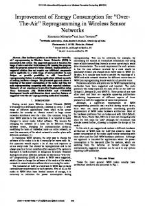
(a) f E (·) and unconstrained

(b) f E (·) and one-hop connection

(c) f E (·) and multi-hop connection

(d) f M I (·) and unconstrained

(e) f M I (·) and one-hop connection

(f) f M I (·) and multi-hop connection

Fig. 1: The impact of constraints on sensors’ motion. The initial positions, trajectories, and final positions are showed with red circles, red solid lines, and black diamonds, respectively. The A2G & A2A links are showed with black solid and dash lines, respectively. TABLE I: Simulation Parameters

∗

random variables hN k+1 xk+1 , and ΣN ∗ ,N ∗ is the covariance N∗ matrix of hk+1 xk+1 ; in the denominator, Σn∗ ,N ∗ ∪n∗ is the ∗ covariance matrix of hnk+1 xk+1 and the set difference between the entire GRF (xk+1 ) and the observations (including the one from sensor n∗ ). Note that the covariance matrices Σn∗ ,N ∗ , ΣN ∗ ,N ∗ , and Σn∗ ,N ∗ ∪n∗ can be constructed from the covariance matrix Qk+1 produced by Kalman filter in Eq. (15). Thereafter, the algorithm updates set N ∗ by adding sensor n∗ . The MC repeats the procedure until all sensors have updated their position for time k + 1. The procedure of MC with MI utility function is presented in Algorithm 2. To summarize, after obtaining the feasible set of positions from NC, the MC returns the next position for each sensor to maximize either the entropy or mutual information gain. V. S IMULATION In this section, the solution proposed in the previous section is examined via simulations. We compare the performances of two different utility functions in three scenarios: unconstrained, one-hop, and multi-hop. The metric of average root mean square error (RMSE) is applied for service time from k = 1 to K: Average RMSE =

K 1  E[(mk − xk )2 ] K

(21)

k=1

where mk is the estimation given by Eq.(15). A list of simulation parameters is shown in Table I. The spatial resolution is the distance between two adjacent locations; and the time resolutions is the difference between time stamps k and k + 1. We plot Fig. 1 as an example of trajectories given by two utility functions in three scenarios, where ASN size is N = 9

Category

Parameter

Value

System

Spatial resolution (m) Time resolution (k) UAV speed (v)

0.3 km 5 min 3.6 km-per-hour

Radio [12]

Ptx for BS / ASN Grx for BS / ASN Receiver noise floor (Pn ) Interference margin (Pi ) Fading margin (Lf ) Bandwidth (B) Minimum uplink capacity (Cmin )

40 dBm / 23 dBm 11.5 dBi / 0 dBi -115 dBm 8 dB 10 dB 10 MHz 1 Mbit/s

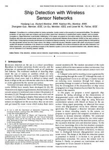
and GRF size is M 2 = 322 . The statistic results of average RMSE of signal reconstruction with an ASN from size N = 6 to N = 18 are presented in Fig. 2. A. Comparing Mobility Strategies in Three Scenarios 1) The Unconstrained Scenario: Under the unconstrained scenario, UAV-carried sensors are allowed to move to any locations within the service area. As illustrated in Fig. 1a, the maximum entropy strategy pushes most of the sensors to the edges of the service area. On the other hand, as illustrated in Fig. 1d, with the maximum mutual information strategy sensors are more evenly distributed. In fact, after a number of iterations, the ASN stabilized at locations which gives an approximate Centroidal Voronoi tessellation (CVT) of the service area. As a results in Fig. 2, the average RMSE given by the MI strategy (blue dash line with cross marker) is much lower than the the average RMSE given by the max entropy

IEEE ICC 2017 Ad-Hoc and Sensor Networking Symposium

Fig. 2: Average RMSEs given by mobility functions f E (·) and f M I (·) with different constraints and number of sensors.

strategy (blue solid line with cross marker). 2) The One-hop Scenario: With the one-hop connectivity constraints, the motion range of the ASN is strictly limited by the communication range of the base station. In this case, there is almost no difference in the results given by two strategies (Fig. 1b and Fig. 1e). No significant gain of average RMSE is achieved by increasing number of sensors from 6 to 18 (the lines with circle marker in Fig. 2). 3) The Multi-hop Scenario: As illustrated in Fig. 1c, the mobility of the ASN is extended significantly. For the max entropy strategy, since the sensors are not able to move to the edge of service area, the average RMSE (solid line with diamond marker in Fig. 2 is actually lower than the same strategy in the unconstrained scenario. However, we know that if the communication range allows the sensors to move to the edges, the performance of maximum entropy in multihop scenario will converge to its performance in unconstrained scenario. For the MI strategy, the ASN is distributed more evenly (Fig. 1f): three sensors are connected to the BS directly in the first tier; each first tire sensor serves as a relay nodes for other two sensors. As a results, the average RMSE given by MI strategy in multi-hop scenario (dash line with diamond marker) is the second lowest of all cases. B. Gain of Performance by Allowing Multi-hop As seen from the Fig. 2, in case of ASN’s mobility is constrained by the connectivity requirements, the difference between two mobility strategies (max entropy and mutual information) is actually minor. On the other hand, we obtain larger performance gain by relaxing the constraint via enabling UAV-to-UAV communications in LTE networks. Our design of NC gives the connection scheme which allows UAVs to pursue more informative measurements and maintain the connectivity at the same time. VI. C ONCLUSIONS AND F UTURE W ORKS In this paper we discussed the path planning for ASNs with connectivity constraints. As it is discussed in previous literatures, in the unconstrained scenario, the maximum mutual information strategy achieved lower RMSE than the maximum entropy strategy. However, we discovered that with the connectivity constrained, the gain of applying better mobility strategy is minor and it is more important to relax the constraints.

By applying the proposed network coordination scheme, we extend the ASN’s mobility via allowing relaying for UAV to base station links. The gain of ASN’s coverage with the multihop communication is significant as the simulation shows. Future research efforts are required for developing reliable ASN applications. When multiple constraints (e.g., energy and connectivity) coexist, k-step path planning is required to avoid driving UAVs to locations where there might be no feasible next positions due to insufficient energy or communication failure. Another interesting problem is to design distributed mechanism for UAVs to exchange data and update their positions, which improves the robustness and scalability of the system. ACKNOWLEDGMENT This work has been supported by the Vinnova GreenIoT project (2015-00347) in Sweden, the National Natural Science Foundation of China (No.61370197). These supports are gratefully acknowledged. R EFERENCES [1] B. V. D. Bergh, A. Chiumento, and S. Pollin, “LTE in the sky: trading off propagation benefits with interference costs for aerial nodes,” IEEE Communications Magazine, vol. 54, no. 5, pp. 44–50, May 2016. [2] Y. Zeng, R. Zhang, and T. J. Lim, “Wireless communications with unmanned aerial vehicles: opportunities and challenges,” IEEE Communications Magazine, vol. 54, no. 5, pp. 36–42, May 2016. [3] X.-Y. Li, P.-J. Wan, and O. Frieder, “Coverage in wireless ad hoc sensor networks,” IEEE Transactions on Computers, vol. 52, no. 6, pp. 753–763, June 2003. [4] Y. Zou and K. Chakrabarty, “Sensor deployment and target localization based on virtual forces,” in INFOCOM 2003. TwentySecond Annual Joint Conference of the IEEE Computer and Communications. IEEE Societies, vol. 2, March 2003, pp. 1293– 1303 vol.2. [5] C. Qiu and H. Shen, “A delaunay-based coordinate-free mechanism for full coverage in wireless sensor networks,” IEEE Transactions on Parallel and Distributed Systems, vol. 25, no. 4, pp. 828–839, April 2014. [6] D. Gu and H. Hu, “Spatial gaussian process regression with mobile sensor networks,” IEEE Transactions on Neural Networks and Learning Systems, vol. 23, no. 8, pp. 1279–1290, Aug 2012. [7] Y. Xu and J. Choi, “Adaptive sampling for learning gaussian processes using mobile sensor networks,” Sensors, vol. 11, no. 3, p. 3051, 2011. [8] N. Ahmed, S. S. Kanhere, and S. Jha, “On the importance of link characterization for aerial wireless sensor networks,” IEEE Communications Magazine, vol. 54, no. 5, pp. 52–57, May 2016. [9] M. Horiuchi, H. Nishiyama, N. Kato, F. Ono, and R. Miura, “Throughput maximization for long-distance real-time data transmission over multiple uavs,” in 2016 IEEE International Conference on Communications (ICC), May 2016, pp. 1–6. [10] D. Simon, Optimal state estimation: Kalman, H, and nonlinear approaches. Hoboken, N.J: Wiley, 2006. [11] A. Krause, A. Singh, and C. Guestrin, “Near-optimal sensor placements in gaussian processes: Theory, efficient algorithms and empirical studies,” J. Mach. Learn. Res., vol. 9, pp. 235– 284, Jun. 2008. [12] Jyrki T. J. Penttinen, The LTE/SAE deployment handbook, 1st ed., Hoboken, NJ, Chichester, West Sussex, 2012.