protecting with sensor networks: perimeters and axes - IEEE Xplore

PROTECTING WITH SENSOR NETWORKS: PERIMETERS AND AXES Stephan Olariu Old Dominion University Norfolk, VA.

Jeffrey V. Nickerson Stevens Institute of Technology Hoboken, NJ.

ABSTRACT

Sensors, in one form or another, have always been a component in physical security systems. Usually such sensors are configured on a perimeter, or perhaps on concentric perimeters. The work was motivated by the realization of the fact that the probability of detecting an intruder is a Quality of Service (QoS) parameter. This implies an interesting trade-off between the amount of resources that a defender can muster and the QoS (in terms ofprobability of detection) that they get. We study this trade-off for a family of structures with an axial design reminiscent of a snowflake. We show that such a structure presents interesting qualities. The relations geometrically deduced in the paper provide a form of sensitivity analysis. The cumulative nature of the detection is discussed and, in addition, a possible implementation in sensor networks is explored. Keywords: physical intrusion, detection probability, Quality-of-Service, wireless sensor networks. INTRODUCTION

There is a wide range of situations that include within them protection problems. For example, banks must protect against bank robbers, and museums must protect against thieves. Adversarial situations often involve two different objectives; on the one hand to protect something important one owns, while, on the other hand, to penetrate and defeat the protection of the opponent. In the field of situation management several ways of reasoning about the environment are discussed and analysed [1]. In order for such schemes to work, it is necessary to categorize the environment and to map corresponding techniques for responding to different identified scenarios. The work reported in this paper is the first step toward a different way of looking at protection-related situations. We are interested in alternative ways of sensing,

leading to better and perhaps different categorization. We are also interested in alternative ways of responding. As part of this paper, we will develop observations about how alternative sensing and protection techniques are related. Our ability to protect often revolves on the way we deploy two different types of resources. The first are sensing resources, and the second are responding resources. Guards in a museum can fulfil both roles - they can see someone attempt to take a painting, and then can intercept the thief. However, in large museums, the tasks are sometimes differentiated. Valuable objects have sensors attached to them, to alert guards that someone may be too close to the object. Readers may notice that the problem bears some resemblance to the class of problems in computational geometry known as the art gallery problems [2]. Usually such problems try to determine a covering set; in our case a covering set would be a set of sensors which guard the entire territory. The association of the art gallery problem to sensor networks has been explored before (e. g. [3-5]) One technology that is available but not yet widely used in situation management and emergency response systems is wireless sensor network technology. It is anticipated that in the near future networked sensors combined with novel data collection and fusion techniques will make monitoring and emergency response systems more accurate and affordable than conventional systems. In this paper we consider a general problem of protection, in which a number of sensor units are to be configured around a central valuable item. We wish to achieve high levels of protection while minimizing the overall cost of the system. Our approach is consistent with others who have observed that security is a QoS issue [6]. The paper is sequenced in the following way. First, a security situation is described, and possible sensor configurations are drawn. Next, the defensive capabilities of one configuration are analyzed. Finally, the results are discussed and conclusions are drawn.

1 of 7

THE SITUATION

We imagine the following situation: m

A valuable item is to be protectedfrom being taken. The item to be protected is in the open, and an intruder may approachfrom any angle. Our problem is to place the sensors in such a way as to minimize cost (the fewer sensors the better) while achieving a high degree of protection. We assume that an intruder at distance at most d from a sensor is sensed and assessed as an intruder with a certain probability that is hardware specific. In the sequel, we consider two models: (1) in the first model the intruder is detected with probability 1 within a disk of radius r centered at the sensor and with probability 0 outside, and (2) in the second model, the intruder is detected with probability 1 inside the above disk and with probability p up to distance d from the sensor. Note that the complexity of the problem lies in the adversarial component. For, the intruder will seek to understand the defenses. Intruders may intentionally attempt to set off sensors in order to figure out their location and capability well before actually attacking [7]. As a result, our job is to provide the negotiated level of resilience with the additional constraint of revealing as little as possible to an intruder.

n

m

n

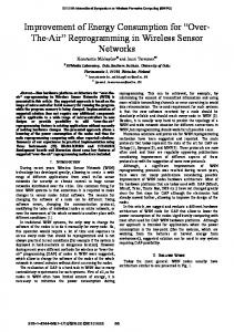
Figure 1. Square or circular concentric perimeter arrangements. There is often an outside perimeter n units away, and an inside perimeter m units away from the center.

-i 4z ^-

I

I

Y

Y

Y

)1

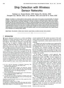
Figure 2. Snowflake defense,

an

axial design.

PERIMETERS AND AXES

A common way to defend against intruders is to create a physical perimeter such as a fence; there are a number of factors to be considered in such a design [8]. In many situations, however, physical perimeters are expensive to construct, and sensor perimeters are used in their stead; for example when one crosses a certain line, a bell rings, which alerts a defender. In high security situations, concentric perimeters are constructed, so that an intruder missed at one perimeter may be caught at the second one (see figure 1). However, perimeters may provide too much information. Through observation or testing, it might be possible for an intruder to figure out exactly where the perimeters are, and therefore to plan more effectively. What alternatives might exist? We might build a structure based on an axial design, such as figure 2. This may go against our intuition initially, as the structure looks easy to penetrate. However, radial structures such as this may provide interesting benefits.

Figure 3. A curved snowflake defense THE BASELINE SCENARIO

The simplest scenario is that of a linear attack performed by an unsophisticated adversary that proceeds in a straight line towards the asset henceforth referred to as the center. -

We

2 of 7

assume

that the defensive infrastructure consists of

sensors placed in the snowflake configuration of Figure 2. The angle between consecutive "branches" of the snowflake is 0, considered to be a system parameter. The choice of 0 is dictated by the amount of resources available and the desired Quality of Service, taken here to mean "probability of detection". Indeed, it is intuitively clear that the larger 0, the less effective the detection. To avoid inconsequential notational complications we assume that 21w is an 0

R(2i-1).

integer.

Each sensor has a sensing radius of r and a transmission range of 2r. To begin, we assume that an intruder at distance at most r from the sensor is detected with probability 1. Later in the paper we shall revisit this assumption. The radius of the circular deployment area is R. We write R = (2+1)r (1) where X is a system parameter that depends on the type of sensors available and on the desired coverage area. For example, in Figure 2, =5 and, consequently, R=llr. It is easy to confirm that, excluding the central sensor, the number of sensors in each branch equals and that the total number of sensors deployed is I2nT I. As an illustra-

(b)

(a)

Figure 4: Illustrating the baseline scenario

Let Di, (i>O) be the event that occurs if some sensor in layer i detects the intruder, assuming that intrusion takes indeed place. It is easy to see that the corresponding probability P[D,] is given by the following expression

2 arcsin P[Di]-

r

R -(2i -)r 0

(3)

c,

+

0

tion, in Figure 2,

0

4

and the total number of

sensors

deployed is 41. The snowflake infrastructure offers a layered protection in a sense that we now define. Referring to Figures 2 and 4(a), the first layer consists of the set of outermost sensors; for every i, i>O, the i-th layer consists of the set of sensors at distance R-(2i-I)r from the center. To orient the reader, we note that the dotted circle in Figure 4(a), contains the sensors in the i-th layer We are interested in evaluating the detection probability offered by the snowflake infrastructure with the above parameters. Referring to Figure 4(b), let 2ai be the angle determined by the two tangents from the center to the sensing disk of a sensor in layer i. Simple trigonometry shows r that sin and, consequently, R - (2i - I)r a

(2)

ai = arcsin

r

R (2i - I)r -

To justify (3) observe that, as illustrated in Figure 4(b), each sensor in layer i "covers" an angle of measure 2a, centered at the asset. Since there are 2fT sensors in layer i, 0

and since the coverage areas are disjoint, they cover a total angle of 2ff (2ai) . Now, the probability of detection is the 0

ratio between the total angle covered and 2m. A somewhat simpler expression of (3) can be obtained by using (1). Indeed, after standard manipulations we obtain 2

P[Di]

arcsin 2(r - i + 1) 0

(4)

Equation (4) captures the essence of the defensive capabilities of the baseline scenario: the probability that the layer i sensors detect intrusion, assuming intrusion occurs, is a function of the density of deployment and the sensing range r of individual sensors. Moreover, the equation can be perceived as offering some sensitivity analysis: indeed, (4) tells us how more protection we obtain by increasing the deployment density and the capabilities of sensors and, conversely, how much protection we loose should we decrease the amount of these resources. For example, we may wonder about the probability of detection offered by

3 of 7

the sensors in the fourth layer in Figure 4. Since -=5, i=4, and 0= equation (4) reveals that P[D4 ] = 0.6434... 4

Importantly, the snowflake infrastructure satisfies the property D1 c D2 c . C Di C ... Consequently, we can write

P[Dj ] < P[D2 ]< ...< P[Dj] < . . .

from which we get easily

j

(5)

It is clear that detection will occur eventually, since the central asset is protected by a collocated sensor (the central sensor). However, in many types of attacks it is not wise to rely on detection by the central sensor. For example, art galleries worry not only about theft, but also about defacement. An important question that has to be answered for the snowflake infrastructure is that of early detection, defined as the identity of the outermost layer k such that P[Dk]=1. Referring to Figure 2 again, we notice that detection is guaranteed in layer 5 as the sensing disks overlap. We now address this important problem in its full generality. As illustrated in Figure 5, P[Dk] 1 is guaranteed to hold as soon as aCk > 0 . Now, replacing this value 2 in (2) we obtain r . 0 (6) sin < 2 R (2k - I)r In turn, (1) and (6) combined yield k 2 -c+i-

be the subscript of the first layer in top-down order for which P[Dj]>.q. Using (4) we obtain qO 1 arcsin 2(r - j + 1) 2 1 * qO -+12 sin 2

THE ENHANCED SCENARIO In real-life applications it is rather unusual for the probability of detection to drop off abruptly from 1 to 0. Rather, as illustrated in Figure 7, the probability of detection is 1 within a disk of radius r centered at the sensor, dropping off to some probability p (strictly less than 1) within a disk of radius d. Notice this is a discrete version of the continuous case where the probability of detection might degrade exponentially with the distance from the center of the sensor. Naturally, p, r and d are system parameters that depend on the actual hardware at hand.

(7)

1 2 sin2

Figure 7: Illustrating detection ranges

k

k

We are interested in evaluating the detection probability at layer i. For this purpose, it makes sense to distinguish between the following cases, illustrated in Figures 8 and 9, respectively.

R-(2k-l)r

Case 1. Neighboring detection disks do not intersect. Figure 6: Illustrating P[Dk] =1

Finally, we are interested in determining the layer that detects the intruder with a given probability at least q. Letj

Referring to Figure 8, let c'i (resp. 3i) stand for the angle determined by the half-line joining the central point (the asset to protect) and the sensor with the tangent to the disk of radius r (resp. d). It is easy to confirm the the angle between the two tangents to the radius d disks is 0 - 2,3i .

4 of 7

saying that detection occurs 1 _ (I _ p)2 = p(2 - p) as claimed.

with

probability

It is not hard to see that in this case the detection probability can be written as P[D ] = 2(l - p)ac, + 2p/3, - p2(O - 2,8,)

0

As before, in case p=O, we obtain the expression in (3), as expected. layer i

Figure 8: Illustrating Case 1

Next, consider a possible attacker. This attacker may come from any of the directions a, b, c, d or e. In each case, the probability of detection is different. To wit, if the attacker comes from directions a or e the probability of detection is 1, if the attacker comes from directions b or d, the probability of detection isp, if the attacker comes from direction c, the probability of detection is clearly 0.

In Figure 9, we looked at a situation where the sensor areas might overlap in coverage. In Figure 10, we look at different concept of overlap. As an intruder moves toward the center, there are several straight paths the intruder can take, akin to the letter-coded directions of figure 8. In direction b or d, the intruder's path will overlap the outer circle of the outermost detector. The probability of detection is p. However, as the intruder continues, the probability of the intruder being detected after crossing through the next detector is now p + (1 - p)p. More generally, the cumulative detection probability at time step t, assuming steps of size 2r, can be thought of as a recurrence relation:

Pt = Pt-1

-

Pt-OP

p1 =P whose solution is

At the risk of some notational overload, we let Di stand for the event that the intruder is detected. It is easy to see that in Case 1, the probability of detection, P[Di], can be expressed as follows )) 2 P[Di 2(1x a + px(fli aip)ai +pfi

0

+(

Pt

a

b

=1-(1-p) c

d

e

0

Of course, in case p=0, we obtain the expression in (3), as expected. Case 2. Neighboring detection disks intersect. We find it convenient to import the notation and terminology established for Case 1 above. Referring to Figure 9, consider again a possible attack from one of the directions a, b, c, d or e. In each case, the probability of detection is different as illustrated next: if the attacker comes from directions a or e the probability of detection is 1, if the attacker comes from directions b or d, the probability of detection isp, if the attacker comes from direction c, the probability of detection is p(2-p). To see this, observe the intruder is not detected with probability (I _ p)2 which amount to

5 of 7

layer i

/R-(2i-)r

Figure 9: Illustrating Case 2

CUMULATIVE DETECTION

Figure 10: Cumulative chances ofdetection as the intruder moves toward the center.

In Figure 10, the intruder crosses four regions of detection probability p before crossing two regions of certain detection. Even for low probability detectors, the situation is not favorable for the intruder; given sensors with a probability of detecting of 1/2, at time step 2 the chances of the intruder evading detection are 25%; at time step 4 they are