ABSTRACT. In this paper, the pattern classification by stochag tic neural networks is considered. This model is also termed as Gaussian mixture model.
Engineering
Industrial & Management Engineering fields Okayama University
Year 1996
Pattern classification by stochastic neural network with missing data Masahiro Tanaka
Yasuaki Kotokawa
Okayama University
Okayama University
Tetsuzo Tanino Okayama University
This paper is posted at eScholarship@OUDIR : Okayama University Digital Information Repository. http://escholarship.lib.okayama-u.ac.jp/industrial engineering/54
Pattern Classification by Stochastic Neural Network with Missing Data Masahiro Tanaka, Yasuaki Kotokawa and Tetsuzo Tanino Department of Information Technology, Okayama University Tsushima-naka 3-1-1, Okayama 700, Jqpan In section 2, the model is defined. In section 3, the learning algorithm is shown. In section 4, a numerical example is shown.
ABSTRACT In this paper, the pattern classification by stochag tic neural networks is considered. This model is also termed as Gaussian mixture model. When missing data exist in the training data, it is the usual custom to remove incomplete instants. Here we take another approach, where the missing elements are estimated by using the conditional expectation based on the estimated model by using the EM algorithm. It is shown by using Fisher’s Iris data that this approach is superior than removing incomplete data.
2. MODEL
Gaussian mixture model has been often used in statistical estimation problems for more than three decades where non-Gaussian distribution is well approximated and the various estimation schemes developed for the Gaussian model can be applied easily.
1. INTRODUCTION
Streit and Luginbuhl [8] proposed the model and the learning scheme in this kind of framework.
For pattern classification, various models have been considered in the field of neural networks. Multilayer neural network with sigmoidal activation function is widely used, where the learning is by “back propagation” (Rumelhart et al. [SI).
Let the classes be expressed as j = l , . .. , M , the problem is to classify n-dimensional real vectors z into M classes. The Gaussian mixture model for the class j(= 1 , ... ,M) is described by
Gaussian function is also used in neural networks. The so called RBF network is usually adopted for function approximations (e.g. [3]), where Gaussian functions are used as the basis functions.
GI
There is another class of neural networks with Gaussian functions, where the network is used for pattern classification. This is called “stochastic neural network”, where the Gaussian functions are used to represent the probability density functions (PDFs) for each pattern class. The simplest way to build stochastic neural networks is to use Parzen window [5]. Gaussian mixture, or also referred to Gaussian sum, has a wide applicability of PDF approximations[7]. The classification is done based on the Bayesian approach, i.e. a vector is judged to belong to the class for which the a posteriori PDF is the largest, i.e. class of z = arg max ,&si(*) -1
where @j = { @ ~ ~ , % ~ I . . . I @ G , } I@,j= { p i j ~ c i j } i denotes the index of the composite Gaussian function and aij is the weight coefficient. ‘
The
elements ‘in
this
model
are
= 1,..sIM}.
In the above expression, the following constraints must be satisfied.
lSr5M
where gi(z) is the probability density function of 2 for the class i , and ,f3j is the prior probability of the class. The parameter estimation scheme was derived by using the EM algorithm [SI.
aij
In this paper, we exploit the stochastic representation of the data for the estimation of missing data based on the conditional expectation formula. 0-7803-3280-6/96/$5.00 O.1996 IEEE
learning
= l,...,Gj,j {a*j,pjj,Z%j;Z
Gi
2 0 Vi,j
.- 1 Vj
ai,
i=l
- 690
-
Cij
> O(positive definite) W , j 3. LEARNING
The EM algorithm is even faster than the gradient descent algorithms [4] (the convergence rate is super linear), but the advantage of the usage of EM algorithm is not only that. It has a nice property that the estimated parameters can easily satisfy the constraints that have to be satisfied, These are satisfied automatically, while in the gradient descent, some additional trick is necessary, e.g. penalty for non-feasible values.
3.1.2 Complete Likelihood and Eh4 Algorithm. The EM algorithm proposed by Dempster et al. [l] is a method when there is a imany to one mapping from some unobservable intermediate variable to the observation and it is effective when the likelihood function for the intermediate variarble is easy to obtain.
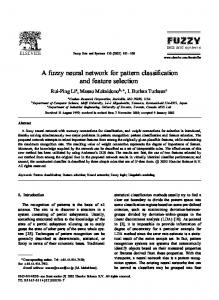
3.1 Estimation of Parameters We derive the learning algorithm based on the EM algorithm. Although the PDF is Gaussian mixture, it is possible to treat that each datum instant is generated from one of the Gaussian sources. This is illustrated in Fig.1. datum
From the stochastic formiula, we have
where Lu(X;Q) = p ( X I 0 ) . Therefore logL(X;8) = logp(X,,qo) - logP(I(X,O) Define Q(Ql0‘) = E [logp(X, IlO)lX, 0’1 Froni Jensen’e inequality E [log P(IIX, S)lX, 0’15 E [log P(ZIX, c3’)IX, 0’1 Hence, by selecting 0 such that &(@IO’) Q(0’10‘) holds, E[logL(X;O)IX,O’] > E[logL(X;O’)IX,0’] is guaranteed.
.:
--.. select one of them with probability
Since P(X1 ZlO) = P(IIO)P(XII,@> the complete likelihood is given by
Fig. 1. Generation of Gaussian mixture data
nn hf
P(X,IIQ)= Thus, if we know the source channel of Gaussian signal, the problem is reduced to the Gaussian problem which has been extensively studied so far. Suppose the channel
ik,j
x = { { 2 k , j ) k =Tli) j = l lM
has generated
ZkJ.
ajai*J,jpikJ,j(zkjIOi,J,j)
j=1 k=l
The conditional expectation is given by
Q(Ql0’) = E [ b p ( X , Il@)lX,W Then, since the unspecified stochastic variable is only Z, we have Q(0lQ’) = logp(X, .TIO)P(IIX, 0’)
Also,
I = { { i k B j } k =Til } J = l M
and further
T = {X,Z} a1 is the a priori probability of the class 1. Let c j , ~be the cost function where the correct class is 1 and the judgement class is j. Then the risk pj(z) for judging the input o to be the class j is given by M
pj
TJ
r
where
*. *
E:=,
*.
.
c::,M::l
By applying the Bayes’ rude, we have cj,ralgl(a)
N
I=1
Thus the decisioifto minimize the risk can be written as j = arg minpj(z) 3
-
hf
3.1.1 Incomplete Likelihood. If the channel that generated x k j for the class j is unknown (i.e. the case when I is unknown), the PDF of X given 0 is the usual likelihood, termed “incomplete likelihood” in
=
n TJ
j = 1 k=1
and
- 691 -
% ,, j( z k j )
wikJ,j(xkj)
Separating I into
=
ikj
xF [ 5
and the other
E's,we have
1
It can be found in the 'commonly used databases
log("ijPij(zkjIOikJ,j))(C p ( I I x , @ ' ) )(e.g. [3]) that missing data is not a special case but
i*,=l
f
=
1% j
k
I\ikJ ( " i j p i j ( Z k j l@ij
)) W : j ( s k j )
i
Hence &(@IO') =
Thus, we restore the missing point based on the estimated model and exploit the partially missing data instants. In the following, how to restore the data is explained.
Tj logpj j
+ 'Ti3 = Qt + Qz + j
k
i
a very common situation.; If we delete all the missing data instants, the amount of available data sometimes become very small and the useful information may be lost.
log("ijPij(zkj loij))w:j(zkj)
First the missing elements of the vector z k j are gathered to the top. The transformation matrix is expressed T k j , with which we have
Q3
where
Tkjzkj
=~ j
~ ~ W : j ( z k j ) l O g P i j ( z k j l e i j ) i b
The problem is to maximize this with respect to 0 =
Since what we want to know is the estimate of we estimate it by
{{~j},{"ij,Pij},Eij}}.
ykj,
(7)
Based on Q(OlO'), we have the following update equations for the parameters. pj
[ 1:; ]
where vkj is a vector of missing elements and the remaining are denoted by % k j .
j = 1 i=l k = l Q3
=
Tj =T
- 692
where E ( " ) [ . ] means the expectation based on the available model at time n. Since P(")(YkjI"kj) =
-
we have E(")[Ykjl z k j ] =
xi a~~)Sglljgi(n)(~llj,'kJ)dvkj J gin)(gkj
xi
1
)dg,j
By some cumbersome matrix manipulations, we have 1 /gy'(vkj,
x exp{-s
(27+n-m)/2
'kj)dgkj =
1 (xkj
lAg)11/2
T
- z;)
1
(~(2n2)l-l( x k j
4. NUMERICAL EXAMPLE
The Fisher's iris data [2] is commonly used for testing the classification algorithms. The data of irises are labelled, which are "Iris selosa (1)" "Iris versicolor (2)" and "Iris verginica (3)". The dataset consists of 4 elements: Sepal length (XI), Sepal zuidlh ( q ) , Petal length (23) and Petal width
- $j)}
(24).
Table 1 shows some statistics of the data.
and
TABLE 1 Statistics of original da.ta 21
where the parameters in the right hand side are the estimated values by the EM algorithm in the current iteration,
3.3 Whole Algorithm Fig. 2 shows the flowchart of the proposed algorithm. The initial model uses random model.
e
1mean Ivalue 23 I 22
"'L
standard deviation
The contribution of this parper is to simultaneously estimate the unknown system parameters ancl the missing data. Thus, we comparre the results of two cases: one is the approach this paper has proposed (Model A) and the other one is to delete the incomplete data instants and estimate the parameters (Model B). First 75 (= 25 x 3) instimces were selected as the learning vector and same number of instances were for the testing. In each experiment, the performances are compared for the models A and B.
initial model
Model A is built with usiing all the learning data by estimating the missing elements.
estimate missing data by eqn. (7) for
Model B is built with data with instances of all the elements existing. By using the model thus obtained, the testing data are evaluated by first int'erpolating the missing elements and next classifying using the model. This evaluation method is the same for Models A and B. In all the corresponding experiments (e.g.Figs. 3,4), the missing instants were supposed to be the same.
&Step (eqn. (1).(6)) for j=I ,....M,k= 1,...,Tj
t Evaluate the test data
t ~
END
Fig. 2. Flowchart of proposed algorithm
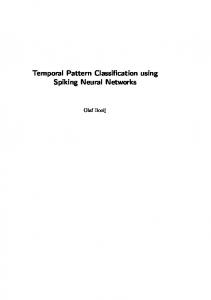
As we can expect that the Model A is generally superior because more information is used, the following results support this hypothesis. In all the following figures, the real lines denote the classificakion error percentages for the learning vectors, and the dashed lines for the test data. Figs. 3 and 4 show the misclassification portion for the learning and test datar by the model wrth kernels ( l , l , l ) ,respectively for thie models A and B, also respectively. Here, about 5% of all the elements were
- 693 -
supposed to be missing. In the 10% case, 25 instants of data were incomplete, thus, a lot of information has to be lost if partially missing datum is to be removed. Figs. 5 and 6 show the results by using (5,5,5) kernels, and Figs. 7 and 8 show the results for 10% case by (5,5,5) model. In the 25% case, 50 instants of data were partially missing.Figs. 9 and 10 show the result for this case. The Model B is inappropriate for such very incomplete data. Model B had a numerical problem for computing ( 6 ) , i.e. the denominator is sometimes 0. This is because, as the learning proceeds with small amount of learning data, the kernel becomes very local (E tends to zero matrix) and thus, there is no Gaussian kernel that covers for many instants of test data. Jo
.
.
.
.
.
.
.
.
/
Fig. 5. Model A (5 kernels, 5% missing)
.
Fig. 6. Model B (5 kernels, 5% missing) Fig. 3. Model A (1 kernel,5% missing) ,
t
.
.
.
.
.
.
.
.
.
Fig. 7. Model A (5 kernels,lO% missing) Fig. 4. Model B (1 kernel,5% missing) It should be noticed that the classification errors are not always monotinically decreasing, rather in many cases, the error rates increase as the learning proceeds. Although it was not shown here, the likelihood function values are always increasing which is the explicit objective function to be maximized. 5 . CONCLUSIONS
Since the objective function was the likelihood function, the learning successfully proceeds as the number of epochs increased. But, with respect to the classification result, the ability of the model attains its best property only at the second or third epoch. As far as
-
Fig. 8. Model B X5 kernels,lO% missing) \
694
-
TABLE 2 Centers of the kernels,
Fig. 9. Model A (3 kernels,25% missing)
___________-------* _ _ _ _ I
--.&-a-=
Fig. 10. Model B (3 kernels,25% missing) we consider the classification problems, this problem has to be extensively studied.
hood training of probabilistic neural networks”, IEEE Trans. Neural Networks, Vol. 5, No. 5,pp. 764-783, 1994. [9]L. Xu and M. I. Jordan,“On convergence properties of the EM algorithm for Gaussian mixtures”, Center for Biological and Computational Learning Department of Brain and Cognitive Sciences, paper No. 111, 1995.
REFERENCES [1]A. P. Dempster, N. M. Laird and D. B. Rubin, “Maximum likelihood from incomplete data via the EM algorithm”, J. Royal Stat. Soc., Vol. B39, pp. 1-38, 1977. [2]R. A. Fisher,“The use of multiple measurements in taxonomic problems” Annals of Eugenics, Vol. 7, pp. 179-188, 1936. [3]J. Moody and C. Darken,“Fast-learning in networks of locally-tuned processing units”, Neural Computation, Vol. 1, pp. 281-294, 1989. [4]P. M. Murphy and D. W. Aha, . UCI Repository of machine learning databases [http://www .ics.uci.ed~/mlearn/MLRepository.html]. Jrvine, CA: University of California, Department of Information and Computer Science, 1994. [5]E. Parzen,“On estimation of a probability density fuction and mode”, Annals of Mathematical Statistics, Vol. 33, pp. 1065-1076, 1962. [6]D. E. Rumelhart, G. E. Hinton and R. J . Williams, “Learning internal representations by error propagation”, in Rumelhart and McCleland eds., Parallel Distributed Processing: Explorations in the Microstructure of Cognition, Vol.1, MIT Press, 1986. [7]D. F. Specht,“Probabilistic neural networks”, Neural Networks, Vol. 3, pp. 109-118, 1990. [8]R. L. Streit and T. E. Luginbuh1,“Maximum likeli- 695 - 1