Pattern Recognition and feature extraction: a

Proceedings of the 6th WSEAS Int. Conf. on NEURAL NETWORKS, Lisbon, Portugal, June 16-18, 2005 (pp109-114)

Pattern Recognition and feature extraction: a comparative study VINCENZO NIOLA Department of Mechanical Engineering for Energetics University of Naples “Federico II” Via Claudio, 21 - 80125 Napoli ITALY

GIUSEPPE QUAREMBA University of Naples “Federico II” Via S. Pansini, 5 – 80131 Napoli ITALY

Abstract: - The selection of features for classifying a pattern by means a fuzzy reasoning, is fundamental in order to obtain a reliable and significative response. The scope of this work is to compare three methods specialized for the extraction of features from images and, consequently, to study the ability of classification performed by applying a fuzzy inference system. The methods to be compared were: Fourier descriptors, Zernike moments and Wavelet coefficients. The best result, in terms of the best performances obtained both as classification reliability and computational time, was represented by the application of wavelet transform. Key-words: - Fuzzy logic, Image analysis, Pattern recognition, Feature selection, Fourier descriptors, Zernike moments, Wavelet coefficients.

1 Introduction The feature extraction is a typical problem of Pattern Recognition (PR), in which the events to be classified are represented by means of images where, in general, the information is distorted for the presence of noise [1]. Sometimes the information is extracted by performing algorithms of Image Analysis (IA) in the case of system based on the vision [2]. Generally, the problem of PR consists of two sub-problems: • to provide an inner representation of input data (i.e., pattern); • to perform a decisional process as well as to assign the pattern to its belonging dominion. In this way, the first problem is to find the pattern, starting from the input data (e.g., image, data stream produced by sensors, etc.) and to produce an inner representation of the pattern as output. This inner representation (often a lot of features extracted from the input data), have to be classified into belonging classes (if there exists).

The problem of recognition, as said before, is faced by means of techniques of IA. The activity of interpretation and analysis of images is a complex operation indeed; in fact the image is simply like a table of gray values (i.e., the gray levels, represented as a matrix of pixel), with added disturbs, called noise, due to electrical instruments. Usually, the activity of interpreting an image is influenced by the typology of the image to be recognized, consequently the choice of algorithms, specifically designed, must take into account such a problem. The aim of this work is to compare three different methods for the calculation of the features to be submitted to a neural network for its training. The data set was composed of 270 images (i.e., 200 pins and 70 nuts) of several dimensions and superficial characteristics (i.e., zinced and burnished), placed in various positions. The 70% of original images, randomly selected, were used for the training set, while 30% for testing set. The images have been made by a digital camera with 3.2 million of pixel, without the use of flash and filter, with a dimension of 640x480 pixel. Calculations were made using Matlab 7.0, The MathWorks, Inc, Natick, Mass.


2 Image Analysis The scope of the Image Analysis is to execute quantitative measures on image in order to obtain a description and, starting from that description, to interpret its content [3]. In general, an image can be thought as a two-dimensional continuous function that associates to a scene its twodimensional representation. For instance, a monochromatic B/W photo can be associated to a function f ( x, y ) ; the value assumed by the function in a point, represents the gray level of the image in that point. By means the technique of digitalization to each pixel is associated a value, that corresponds to the average value of gray in the corresponding area (i.e., quantization). The aim of PR is to represent a digitalized image by a finite set of features extracted from the same image. A feature, as said before, could be an object of high level: a geometrical descriptor of a region of the image or a geometrical object in 3D. The features can be represented as continuous, discrete or binary functions. However it must notice: • the process of feature extraction requires time consuming for the calculation; • the extracted features could contain errors, due to noise or an erroneous application of algorithms. The process of selection of features is one of the key problems for every system dedicated to the pattern recognition and it consists to decide which features to use, among all those available ones, for a specific problem. It is important, for a reliable solution of such systems, to choose (and therefore to extract) features such that they: • are important for the problem; • are computing realizable; • give the minimum number of misclassifications; • reduce the problem to a minimum number of data without loss of information. Sometimes a mathematical approach can help us to choose the most appropriate features, in other cases it could be more useful to perform some simulations. However, many times the choice is based on the experience. As the features are grouped in array of n dimensions the space, in which the problem is involved, is represented by

recognition, multi-class classification and data compression tasks, e.g. speech recognition, image processing or customer classification. As supervised method, LVQ uses known target output classifications for each input pattern of the form . The main idea is to cover the input space of samples with ‘codebook vectors’ (CVs), each representing a region labelled with a class. A CV can be seen as a prototype of a class member, localized in the centre of a class or decision region (‘Voronoї cell’) in the input space. As a result, the space is partitioned by a ‘Voronoї net’ of hyperplanes perpendicular to the linking line of two CVs (mid-planes of the lines forming the ‘Delaunay net’. A class can be represented by an arbitrarily number of CVs, but one CV represents one class only. In terms of neural networks a LVQ is a feed-forward net with one hidden layer of neurons, fully connected with the input layer. A CV can be seen as a hidden neuron (‘Kohonen neuron’) or a weight vector of the weights between all input neurons and the regarded Kohonen neuron respectively

3 Mathematical background 3.1 Zernike moments The moments and functions of moments have been used in order to obtain features in numerous PR applications applied to two-dimensional images [7]. Since 1961 the moment invariants were introduced by using a linear combination of regular moments [8]. These not linear functions have the property of being invariant for translation, rotation and scale. Since such features capture total information on the image, than they have to be applied to the entire image. Let be f ( x, y ) a continuous intensity function of the image in a point ( x, y ) ; the regular moments m pq of order ( p + q) are defined as [7]: ∞ ∞

m pq =

p

y q f ( x, y )dxdy

(1)

−∞ −∞

{ p, q = 0,1, 2,K , ∞}

where . In order to make the moments invariant to translation, central moments are defined as follows:

Rn . The key point of IA is the automatic recognition of an object in a scene, independently from its position, dimension and direction. Learning Vector Quantisation (LVQ) is a supervised version of vector quantisation, similar to SelfOrganizing Maps (SOM) based on work of [4], [5] and[6] for a comprehensive overview). It can be applied to pattern

∫ ∫x

∞ ∞

µ pq =

∫ ∫ (x − x)

−∞ −∞

where

p

( y − y )q f ( x, y )dxdy

(2)


x=

m10 , m00

m01 , m00

y=

( p, q = 0,1, 2,K , ∞ ) .

The point ( x , y ) , calculated with (1), is the centroid of the image. By means of linear combination of moments several not linear functions can be derived, invariant for translation, scale and rotation [9]. The central moments normalized become invariant for scale [8], [9]:

µ pq p+q , γ= +1 γ µ00 1

η pq =

where { p + q = 3, 4,5,K , ∞} . A non linear set of functions, invariant for rotation, translation and scale, are the following [8]:

ζ 1 = η 20 + η02 ζ 2 = (η 20 − η02 ) + 4η112 2

ζ 3 = (η30 − 3η12 ) + ( 3η 21 − η03 ) 2

ζ 4 = (η30 − η12 ) + (η 21 + η03 ) 2

{ ( ) , i = 1,K, 4} .

{m

pq

base

of

Jain

}

p, q = 0,1,K , ∞ show

Theorem

[3]

Z nm =

π

ki   ck exp  2π j  N N  k =− +1

∑ 2

the

moments

the property to represent

2π 1

zi =

N 2

The inverse relationship exists between c (k ) and z (i ) :

uniquely the image. Teague [10] suggested the use of orthogonal moments, based on the theory of orthogonal polynomials in order to eliminate the problem associated with regular moments, which show a redundancy due to the fact that the basis x p y q is not orthogonal. He introduced the Zernike Moments as:

n +1

In the other side, the Fourier descriptors [3], are applied exclusively to the contour of the object to be recognized; it makes more sensitive to the noise and the perturbations showed by the contour. Based on a Fourier analysis technique applied to the boundary coordinates of an object expressed as complex numbers, Fourier descriptors are widely used in image processing to describe and classify shapes. The shape descriptors generated from the Fourier coefficients numerically describe shapes and can be normalised to make them independent of translation, scale and rotation. Classification is performed by comparing descriptors of the unknown object with those of a set of standard shapes, finding the closest match [11]. [12] introduced Fourier descriptors using complex representation in 1972. This method ensures that a closed curve will correspond to any set of descriptors. The shape is described by a set of N vertices { z (i ) : i = 1,K , N } corresponding to N points of the outline.

2

logarithm is assumed: log ζ i the

3.2 Fourier descriptors

coefficients of the Fourier transform of z :

In many applications, in order to avoid the overflow, the

On

.

The Fourier descriptors {c(k ) : k = − N / 2 + 1,K , N } are the

.

2

0 ≤ m ≤ n, n − m = even, n > 0

ck =

1 N

N

∑z i =1

i

ik   exp  −2π j  N 

The range of k can be restricted to

{− N 72 + 1, N / 2} :

according to Shannon’s theorem, the highest frequency is obtained for k = N / 2 , and any c (k ) with k greater than N / 2 would be redundant since we use a discrete representation of the outline.

∫ ∫ V ( r,θ ) ∗ f ( r cos θ , r sin θ ) rdrdθ nm

0 0

where

 y r = x 2 + y 2 , θ = tan −1   , − 1 < x, y < 1 , x with m, n integer values;

3.3 Continuous Wavelet Transform The wavelets used in this paper are those proposed by [12] She constructed a series of mother wavelets (indexed by N and denoted by dbN) with each mother in the series having regularity proportional to N [14]. Each Daubechies' wavelet are compactly supported in the time domain. Typically wavelets of class mr are specifically constructed so that some properties are verified [15].


A mother wavelet ψ is a function of zero h-th moment:

To show the above mentioned property, it is sufficient to expand the function in Taylor series. An example of wavelets is given by Daubechies’ family {dbN, N = 1, 2, …} [16]). It is

+∞

∫ x ψ ( x)dx = 0 ,

h ∈ N.

h

−∞

supp φ ⊆ [0, 2N − 1] , supp ψ ⊆ [0, 2N − 1]

From this definition, it follows that, if ψ is a wavelet whose all moments are zero, also the function ψjk is a wavelet, where

and

ψ jk ( x) = 2 j / 2ψ (2 j x − k ) .

+∞

∫ x ψ ( x)dx = 0 , h

In fact, we have +∞

∫2

j/2

Moreover, there is the following smoothness property: for any N > 2, the D2N wavelets verify

x hψ (2 j x − k )dx =

−∞

+∞

= 2j/2 =

=

h = 0, 1,…, N − 1.

−∞

h

1  y+k ∫−∞ 2 j  2 j  ψ ( y)dy =

φ, ψ ∈ HλN,

0.1936 ≤ λ ≤ 0.2075,

2 j/2 2 j ( h +1)

+∞

where HλN is the Hölder smoothness class with parameter λ.

−∞

3.3.1 Two-dimensional Wavelets Let us consider a two dimensional function f ( x, y ) which are

2 j/2 2 j ( h +1)

 h  h − m +∞ m ∑  k ∫ y ψ ( y)dy =0. m=0  m  −∞

square integrable over the real plane: f ( x, y ) ∈ L2 ( R 2 ) . A

h ∫ ( y + k ) ψ ( y)dy =

h

wavelet basis for L2 ( R) is to take the simple product of onedimensional wavelet:

Moreover, consider a wavelet ψ and a function φ such that {{ ϕ j0k }, {ψjk}, k ∈ Z, j = 0, , 2,…} is a complete orthonormal system. By Parseval theorem, for every f∈ L (R), it follows that

Ψ j1 j2k1k 2 ( x, y ) = ψ j1k1 ( x ) ψ j2k 2 ( y )

2

j1

f (t ) = ∑ a j0kϕ j0 k (t ) + ∑ ∑ d jkψ jk (t ) j = j0

k

k

.

It is easy to show that Ψ ’s as defined above are indeed wavelets and that they form an orthonormal basis for L2 ( R) . It can been show that the “detail space” W j is itself made up of three orthogonal subspaces as follows:

Ψ 1 ( x, y ) = ϕ ( x)ψ ( y );

The decomposition of a function f (t ) by wavelet (i.e., the CWT) is represented by the following detail function coefficients: +∞

d jk =

∫ s(τ ) ⋅

−∞

1 2

j

τ − k  dτ j   2 

ψ

and by the approximating scaling coefficients

.

Ψ 2 ( x, y ) = ψ ( x) ϕ ( y ); Ψ 3 ( x, y ) = ψ ( x)ψ ( y ). Mallat [16] notes that the three sets of wavelets correspond to specific spatial orientations: the wavelet Ψ1 corresponds to the horizontal direction, the wavelet Ψ 2 with the vertical direction and Ψ 3 with the diagonal.

+∞

a j0 k =

∫ s(τ ) ⋅ψ (τ − k )dτ

−∞

Note that djk can be regarded, for any j, as a function of k. Consequently, it is constant if the function f (t ) is a smooth function, having considered that a wavelet has zero moments.

4 Results The hardware used for the study was not particularly expensive or specialized for the image analysis. For every image of training set the features were calculated by applying the methods exposed in the previous paragraph. For giving a


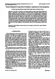
total appraisal on the reliability of recognition, several testing sessions have been executed; the following parameters were estimated: • recognition factor, denoted with ρ , estimates the efficiency of the recognizer, calculated as: # objects correctly recognized/# objects analyzed; • computational time: expressed in seconds, the time occurring for the identification of the object; • memory occupation; • number of features necessary for a complete inner representation of the pattern, indicated as Ftot. Since the first three parameters are depending from Ftot, it is important to investigate mainly on Ftot and to express the results of the parameters that we want to estimate by means this value. An example of grouped objects is shown in the Fig.1. Note that the background was black, the objects were randomly positioned while their surface was zinced or burnished.

100.00 95.00 90.00

Fourier

% 85.00

Zernike

80.00

Wavelet

75.00 70.00 0.10

0.20

0.30

Learning rate

Fig.3 Percentage of recognition for various learning rate (10 neurons)

100.00 95.00 90.00

Fourier

% 85.00

Zernike

80.00

Wavelet

75.00 70.00 Methods of recognition

Fig.4 Test Set ( α = 0.1 ): percentage of recognition

Fig.1 An example of grouped pins and nuts The methods were tested in several conditions: number of neurons and learning rate of LVQ; the responses are reported in the Fig.2 and 3 respectively. The total percentage of recognition for each method is reported in Fig.4.

The results presented, were obtained by using a vector composed of 10 features. In the Tab. 1 below, are compared the computational time occurred for the identification of 30 objects, disposed in several positions, belonging to the Training Set, with reference to the applied method. Method Fourier descriptors

100,00 95,00 90,00

Fourier

% 85,00

Zernike

80,00

Wavelet

Zernike moments Wavelet coefficients

Computational time (s) 72 108 215

Tab. 1 Comparison of computational time

75,00 70,00 10

20

30

5 Conclusions

Number of neurons

Fig.2 Percentage of recognition for various neurons ( α = 0.1 )

A comparative study (both analytical and experimental) on the recognition rate for different extraction methods was performed. The comparison of three methods for detecting the pattern of several objects, showed the reliability and the robustness of wavelet coefficients in order to the pattern recognition. The wavelet application seems to represent the


best compromise among the factors indicating the performance of a complete system of Image Analysis. The results reached, compared with the ones obtained by means of other methods, demonstrates the validity of this choice. Since the training session is fast and easy, the neural networks are ideal in order to solve problems of pattern recognition. At this stage of the study we considered not important to choose a batter neural network, in fact, in particular it should be more stimulating and interesting to study, in the future, the problem of pattern recognition in the case of imprecise or noised images in conjunction with the wavelet transform. The response, in terms of percentage of recognition, was also experimentally studied for several learning rates and number of neurons of LVQ. An application of the proposed net for object extraction based on noisy scenes is also tested. The recognition rate is quite stable if compared with various learning rate and number of neurons employed in the LVQ. Probably this is due to the fact that the noise was not added to the scenes. A complete investigation will be need in order to take into account higher dimensional feature space in presence of noised images.

References: [1] Jeffrey D. Ullman: Pattern Recognition Techniques. Butterworths, London, 1973. [2] Richard Watson: A survey of gesture recognition techniques. Technical report, Dep. of Computer Science, Trinity College, Dublin, 1993. [3] A.K. Jain, Fundamentals of Digital Image Processing, Prentice Hall, 1989. [4] Y. Linde, A. Buzo, and R. Gray, "An algorithm for vector quantizer design," IEEE Trans. Commun., vol. 28, pp. 84--95, Jan. 1980 [5] Gersho A. and Gray R.M., (1992), Vector Quantization and Signal Compression. Kluwer Academic Publishers. [6] Kohonen, T.; The Self-Organizing Map, Procs. IEEE, 78, 1464 ss, 1990. [7] C. Teh and R. T. Chin. On image analysis by the methods of moments. IEEE Trans. on Pattern Analysis and machine Intellig., 10:496-512, July 1988. [7] M. K. Hu. Pattern recognition by moment invariants. In Proc. IRE, number 49, Sept. 1961. [8] T. H. Reiss. Recognizing Planar Objects Using Invariant Image Features. Springer-Verlag, 1993. [9] M. Teague. Image analysis via the general theory of moments. J. Opt. Soc. Am., August 1980 [10] Keyes, L. and Winstanley, Adam C. (1999) Fourier Descriptors as A General Classification Tool for

Topographic Shapes. In Whelan, Paul F., Eds. Proceedings Irish Machine Vision and Image Processing Conference, pages 193-203, Dublin City University. [11] G.H. Granlund, "Fourier Pre-processing for hand print character recognition", IEEE Trans. Computers, Vol C-21, Febr. 1972, pp. 195-201. [12] Daubechies I., Ten Lectures on Wavelets, SIAM, 1992. [13] Strang G. and Nguyen T.: Wavelets and Filter Banks. Wellelsley-Cambridge Press, 1996. [14] Meyer Y.; Wevelets and Operators – Cambridge: Cambridge University Press, 1992. [15] Härdle, W. et al 1998. Lecture Notes in Statistics: Wavelets, approximation and statistical applications. New York: Springer. [16] S. Mallat (1989), A theory for multiresolution signal decomposition: the wavelet representation”, IEEE Pattern Anal. And Machine Intell. Vol. 11 n. 7 pp 674693.