AUTOMATED INSPECTION
Pattern recognition in the automatic inspection of aluminium castings D Mery, R R da Silva, L P Calôba and J M A Rebello
In this paper, we report the results obtained recently by analysing around 400 features measured from 23,000 regions segmented in 50 noisy radioscopic images of cast aluminium with defects. The extracted features are divided into two groups: geometric features (area, perimeter, height, width, roundness, Fourier descriptors, invariant moments, and other shape factors) and grey value features (mean grey value, mean gradient in the boundary, mean second derivate in the region, radiographic contrasts, invariant moments with grey value information, local variance, textural features based on the co-occurrence matrix, coefficients of the discrete Fourier transform, the Karhunen Lòeve transform and the discrete cosine transform). We propose a new contrast feature obtained from grey level profiles along straight lines crossing the segmented potential defects. Analysing the area Az under the receiver operation characteristic (ROC) curve, this feature presents the best individual detection performance yielding an area Az=0.9941. In order to make a compact pattern representation and a simple decision strategy, the number of features is reduced using feature selection approaches. The relevance of the selected features is evaluated by the calculation of a linear correlation coefficient. The results are shown in Tables of the linear correlation coefficients between features, and among features and class of defect. In addition, statistical classifiers and classifiers based on neuronal networks are implemented in order to establish decision boundaries in the space of the selected features which separate patterns (our segmented regions) belonging to two different classes (regular structure or defects).
1. Introduction Automatic detection of failures in non-destructive testing is normally carried out by a pattern recognition method, the steps of which are illustrated in Figure 1, image formation, pre-processing, segmentation, extraction of features, and classification (Mery et al, 2003a). Each of these steps is briefly presented below. ∑ Image Formation: The images are obtained by X-ray irradiation of the test-piece. The X-rays are then converted to a visible image by means of an image amplifier or a flat-panel detector that are sensitive to X-rays. The sensor is bi-dimensional (or uniDomingo Mery is in the Departamento de Ingeniería Informática, Universidad de Santiago de Chile, Av. Ecuador 3659, Santiago de Chile. E-mail:
[email protected]; web: http://www.diinf.usach.cl/~dmery Romeu R da Silva and João M A Rebello are at Engenheria Metalurgica e de Materiais, Escola de Engenharia e COPPE, Universidad Federal do Rio de Janeiro, PO Box: 68505, CEP 21945-970, Rio de Janeiro. E-mail: {romeu,jmarcos}@metalmat.ufrj.br; web: http://www.metalmat.ufrj.br Luiz P Calôba is at Engenheria Eletronica, Escola de Engenharia e COPPE, Universidad Federal do Rio de Janeiro, PO Box: 68504, CEP 21945-970, Rio de Janeiro. E-mail:
[email protected]; web: http: //www.lps.ufrj.br
Insight Vol 45 No 7 July 2003
dimensional in motion) in order to capture the two dimensions of the image. An A/D converter turns the electrical signal into binary code that can be interpreted by a computer to form a digital image of the study object. ∑ Pre-processing: This stage is devoted to improving the quality of the image in order to better recognise flaws. Some of the techniques used in this stage are elimination of noise by means of digital filters or integration, improvement of contrast, and restoration. ∑ Segmentation: The segmentation process divides the digital image into disjoint regions with the purpose of separating the parts of interest from the rest of the scene. Over the last few decades, diverse segmentation techniques have been developed. These can largely be divided into three groups: pixel, edge and region orientated techniques. The present investigation uses the segmentation process oriented towards the detection of edges by employing the LoG filter (Mery and Filbert, 2002b). As can be seen in Figure 2, this technique searches for changes in the grey values of the image (edges), thus identifying zones delimited by edges that indicate flaws. ∑ Feature extraction: In the inspection of cast pieces, segmentation detects regions that are denominated as ‘hypothetical defects’, which may be flaws or structural features of the object. Subsequently the feature extraction is centred principally around the measurement of geometric properties (area, perimeter, form factors, Fourier descriptors, invariant moments, etc.), and on the intensity characteristics of regions (level of grey, gradient, second derivative, texture features, etc.). It is important to know which features provide information about flaws. To this end, a feature selection is carried out to find those features that best describe flaws (eliminating for example features that are correlated or provide no information whatsoever) (Jain et al, 2000). ∑ Classification: Finally, classification orders segmented regions in specific regions according to extracted features, assigning each region to one of a number of pre-established groups, which represent all possible types of regions expected in the image. Typically the classes that exist in detection of flaws in cast pieces are two: ‘defects’ or ‘regular structures’1. It must be noted that a classifier is designed following a supervised training. During this stage a statistical study is carried out of the features of flaws extracted from objects whose flaws are known a priori. Simple classifiers can be implemented by comparing measured features with threshold values; nonetheless it is also possible to use more sophisticated classification techniques such as those that carry out statistical and geometric analyses of the vector space of the features, or those that employ neuronal networks or fuzzy logic (Castleman, 1996; Jain et al, 2000; Mery and Filbert, 2002b). This paper presents an exhaustive analysis of over 400 features extracted from over 23,000 regions in 50 noisy radioscopic images. The paper is organised as follows. Section 2 briefly describes the features used. Section 3 carries out a feature selection in order to reduce computational cost of classification. Section 4 presents 1
A sub-classification of flaws is possible to determine the type of flaw.
1
Figure 1. Pattern recognition in the automatic detection of flaws
Figure 2. Detection of flaws using edge detection: (a) original image, (b) second derivative, (c) edges using a LoG filter (d) and (e) detection of flaws
the linear correlation method for the selected features. Section 5 shows the results obtained by using statistical classifiers and classifiers based on neuronal networks, using original features and those obtained by an analysis of principal components. Finally, conclusions and suggestions for future research are presented2.
2. Feature extraction As mentioned above, segmentation is performed using an edge detection technique. All regions enclosed by edges in the binary image are considered ‘hypothetical defects’ (see example in Figure 3). During the feature extraction process the properties of each of the segmented regions are measured. The idea is to use the measured features to decide whether the hypothetical defect corresponds to a flaw or a regular structure. The features extracted in this investigation are described below, and have been grouped in two categories: geometric (geo) and intensity (int) features. Geometric features provide information relative to the size and form of the segmented hypothetical flaws. Intensity features, on the other hand, provide information about the grey value of the segmented regions. Table 1 presents the set A summarised version of this paper is presented at the International Symposium on Computed Tomography and Image Processing for Industrial Radiology, June 23-25, 2003, Berlin, Germany. A Spanish version of this paper is available in (Mery et al, 2003). 2
2
of features used in this investigation. The details of how these are calculated can be found in the references. The total number of features extracted is 405 divided into 37 geometric features, and 368 intensity features.
3. Feature selection In order to reduce the computational time required for classification it is necessary to select features; this way the classifier only works with non-correlated features that provide flaw detection information. There are a variety of methods for evaluating the performance of the extracted features. The present Section includes the ROC analysis and the Fisher discriminator while the following Section explains the linear correlation analysis. The ROC (receiver operation characteristic) analysis is commonly used to measure the performance of a two-class classification. In our case, each feature is analysed independently using a threshold classifier. This way, a hypothetical flaw is classified as a ‘regular structure’ (or ‘defect’) if the value of the feature is below (or above) a threshold value. The ROC curve represents a ‘sensitivity’ (Sn) versus ‘1-specificity’ (1-Sp), defined as:
Sn =
TP TP + FN
1 - Sp =
FP .................(1) TN + FP
Insight Vol 45 No 7 July 2003
Table 1. Extracted features Type
Variable
#
Description
Ref
geo
I
1
geo
(i , j )
2-3
number of the image centre of gravity
Castleman, 1996
geo
h, w
4-5
height and width
Castleman, 1996
geo
A, L
6
area and perimeter
Castleman, 1996
geo
R
8
roundness
Castleman, 1996
geo
f1 ... f7
9-15
Hu’s moments
Sonka et al, 1998
geo
DF0 ... DF7
16-23
Fourier descriptors
geo
FM1 ...FM4
200
Flusser and Suk invariant moments
Sonka et al, 1998
geo
FZ1 ... FZ3
204-206
Gupta and Srinath invariant moments
Sonka et al, 1998
geo
(ae,be)
207-208
major and minor axis of fitted ellipse
Fitzibbon et al, 1999
geo
ae/be
209
ratio major to minor axis of fitted ellipse
Fitzibbon et al, 1999
orientation of the fitted elipse
Fitzibbon et al, 1999
Zahn & Roskies, 1971
geo
a
210
geo
(i0,j0)
211-212
geo
Gd
213
Danielsson form factor
int
G
24
mean grey value
int
C
25
mean gradient in the boundary
Mery & Filbert, 2002b Mery & Filbert, 2002b
centre of the fitted ellipse
Fitzibbon et al, 1999 Danielsson, 1978 Castleman, 1996
int
D
26
mean second derivative
int
K1 ... K3
27-29
radiographic contrasts
int
Ks
30
deviation contrast
Mery & Filbert, 2002b
int
K
31
contrast based on CLP3 at 0° and 90°
Mery & Filbert, 2002b
int
DQ
32
difference between maximum and minimum of BCLP3
Mery, 2003
int
D'Q
33
ln(DQ +1)
Mery, 2003
int
sQ
34
standard deviation of BCLP3
Mery, 2003
int
D"Q
35
DQ normalised with average of the extreme of BCLP3
Mery, 2003
int
Q
36
mean of BCLP3
Mery, 2003
int
Kamm, 1998
F1 ... F15
37-51
first components of DFT of BCLP3
int
f'1 ... f'7
52-58
Hu moments with grey value information
int
s g2
59
int
Tx1
60-87
mean and range of 14 texture features4 with d=1
Haralick et al, 1973
int
Tx2
88-115
mean and range of 14 texture features4 with d=2
Haralick et al, 1973
int
Tx3
116-143
mean and range of 14 texture features4 with d=3
Haralick et al, 1973
int
Tx4
144-171
mean and range of 14 texture features4 with d=4
Haralick et al, 1973
int
Tx5
172-199
mean and range of 14 texture features4 with d=5
Haralick et al, 1973
int
YKL
214-277
64 first components of the KL transform5
Castleman, 1996
int
YDFT
278-341
64 first components of the DFT transform5
Castleman, 1996
int
YDCT
342-405
64 first components of the DCT transform5
Castleman, 1996
local variance
Mery, 2003 Sonka et al, 1998 Mery & Filbert, 2002b
in which TP is the number of true positives (correctly classified defects), TN is the number of true negatives (correctly classified regular structures), FP is the number of false positives (false alarms, or regular structures classified as defects) and FN false negatives, (flaws classified as regular structures)6. A graphic CLP: Crossing line profile, grey value function along a line that crosses the region at its centre of gravity. The term BCLP refers to the best t CLP, in other words the CLP that presents the best homogeneity at its extremes (Mery, 2003). 4 The following features are extracted based on a co-ocurrence matrix: second angular moment, contrast, correlation, cum of squares, inverse difference moment, mean sum, variance of the sum, entropy of the sum, entropy, variance of the difference, entropy of the difference, 2 measures of correlation information, and maximum correlation coefficient, for a distance of d pixels. 5 The transformation takes a re-sized window of 32 ¥ 32 pixels which includes the region and its surroundings. 6 In the literature the following terms are also known False Acceptance Rate (FAR) and False Rejected Rate (FRR) defined as 1-Sp and 1-Sn respectively (Jain et al, 2000; Mery and Filbert, 2002a).
representation is presented in Figure 4. Ideally, Sn = 1 and 1-Sp = 0, this means that all defects were found without any false alarms. The ROC curve makes it possible to evaluate the performance of the detection process at different points of operation (as defined for example by means of classification thresholds). The area under the curve (Az) is normally used as a measure of this performance as it indicates how flaw detection can be carried out: a value of Az = 1 indicates an ideal detection, while a value of Az = 0.5 corresponds to random classification (Egan, 1975). Another method for evaluating classifier performance is the Fisher discriminator, which evaluates the following function:
(
J = spur C -w1C b
.................................(2)
where Cb and Cw represent the selected features’ interclass (between) and intraclass (within) covariances respectively. A large value for J indicates a good separation of classes as it ensures a small intraclass variation and a large interclass variation in the feature space (Fukunaga, 1990). The results presented in this article are derived from the analysis of 50 radioscopic images of cast aluminium pieces. The images have a high noise component due to the fact that they were taken without using integration techniques in which various images of the same scene are averaged to increase the SNR. In these images a total of 22,936 regions were segmented. Visual inspection determined that 60 of these were real flaws corresponding to blow holes in the piece. These flaws were located in areas of the piece in which detection is very difficult (see examples in (Mery and Filbert, 2002b)). The 405 features mentioned in Table 1 were extracted from each one of the almost 23,000 regions. A pre-selection of features was obtained by eliminating those that presented an area under the ROC curve Az< 0.8 and a Fischer discriminator J < 0.2 Jmax, where Jmax corresponds to the maximum Fisher discriminator obtained upon evaluation of each of the features. Additionally, if two features present a correlation coefficient with an absolute value greater than or equal to 0.95 then the feature with a lower Az is eliminated. In this manner of the 405 features, 376 were eliminated. Table 2 shows the 28 pre-selected features. As can be seen, the best results were obtained with features belonging to the contrast family. Texture also performed well. Additionally, some of the features were geometric, although better results were obtained with intensity features. Figure 5 shows the best ROC curve obtained for F1, the contrast feature based on a Fourier analysis of grey values along the straight lines that cross the regions (Mery, 2003). In this case the area under the curve is Az = 0.9944. The good class separation offered by this feature can also be appreciated. Following the pre-selection of features a selection process was carried out based on the Sequential Forward Selection (SFS) method (Jain, et al, 2000). This method requires an objective function f that evaluates the performance of the classification using m features. This function could be, for example, the Fisher discriminator defined in Eq. (2). The method begins with one feature (m =1), and a search is performed for the feature that maximises the function f. Subsequently, a second search is carried Table 2. Values of the area under the ROC curve Az and Fischer discriminator J for the 28 pre-selected features #
var
#
var
4
h
0.94 1.5
59
s
0.95 1.8
139
Tx3 0.87 1.5
186
Tx5 0.96 3.9
8
R
0.91 2.0
85
Tx1 0.93 2.9
156
Tx4 0.92 1.9
190
Tx5 0.90 1.5
25
C
0.93 2.0
87
Tx1 0.83 1.9
162
Tx4 0.89 1.4
195
Tx5 0.94 3.0
30
Ks
0.99 3.0
100
Tx2 0.97 4.6
167
Tx4 0.91 2.2
208
be
31
K
0.99 6.8
101
Tx2 0.83 1.6
170
Tx4 0.90 1.9
285 YDFT 0.96 1.4
Az
J
3
Insight Vol 45 No 7 July 2003
)
2 g
Az
J
#
var
Az
J
#
var
Az
J
0.96 1.7
33
D'Q 0.99 4.6
113
Tx2 0.92 2.5
179
Tx5 0.97 3.6
360 YDCT 0.95 2.5
37
F1
0.99 1.9
128
Tx3 0.96 3.2
182
Tx5 0.94 2.8
376 YDCT 0.94 1.7
3
Figure 3. Example of a region. (a) X-ray image, (b) segmented region, (c) 3d representation of the intensity (grey value) of the region and its surroundings
Figure 4. Defect Classification. a) Distribution of classes using a single feature x. b) Confusion matrix. c) ROC curve varying the threshold q
out for that feature that maximises the function f with two features (m =2). This method ensures that neither features that are correlated with the already selected feature nor those that do not maximise f are considered. This process is repeated until the best n features are obtained. This approach works best with normalised features, ie those that have been linearly transformed in such a way as to obtain a mean value equal to zero, and a variance equal to one. It is also possible to use another objective function to evaluate separation between classes. An alternative function would be to evaluate the specificity for a threshold classification that obtains a sensitivity of 100%, known in the literature as Sp @ Sn=100%. The first 10 features selected with the SFS method are shown in
4
Figure 6 for both objective functions. As can be seen the objective function increases in the measure that new features are added with the SFS method. For example, and using only one feature, feature # 31 (K) maximises function J, thus obtaining a value of J=6.8 (see first column in Figure 6(a)). Likewise, when using this feature with feature # 101 (Tx2) the objective function J increases to 8.5 (see second column in Figure 6(a)). It should be mentioned that this texture is the feature that most increases J in combination with feature K. This process is repeated until the 10 best features are found. It can be concluded that there are a number of selected features that show a significant performance. An appropriate mixture of
Insight Vol 45 No 7 July 2003
Figure 5. ROC curve and class distribution for the best contrast feature (# 37)
(a) (b) Figure 6. Selection of the first 10 features 10 by means of the SFS method using a) Fisher discriminator (J) and b) sensitivity specificity = 100%
contrast and texture features obtains the best separation of classes. When designing a classifier it is also necessary to consider the computational cost of calculating the features. It is recommended that the selected features should be able to be computed quickly in order that the detection of flaws can be carried out in the time required for the automated inspection process.
4. Linear correlation analysis The analysis of the two linear correlation coefficients is a method for evaluating the correlation that exists between selected features, and also the correlation between features and the ideal classification supervision variable yk, in which yk is 1 (or 0) if the sample k belongs to the class ‘defect’ (or ‘regular structure’). A detailed explanation for calculating linear correlation coefficients is given in (Silva et al, 2002a). In the present investigation, after the pre-selection of the 28 most relevant features according to the Fisher and ROC criteria, (summarised in Table 2), a linear correlation analysis was performed on a set of the 60 existing samples from the
Insight Vol 45 No 7 July 2003
‘defective’ class, and 180 randomly selected samples taken from 22,786 samples belonging to the ‘regular structure’ class. The limiting value for a variable to have a 95% probability of being correlated with another is given by 2 N where N is the number of samples of the variable (Silva et al, 2002a). Thus the limiting values are 2 60 = 0.26 for correlation in the ‘defect’ class, and 2 180 = 0.15 for correlation in the ‘regular structure’ class, while for correlation between classes the limiting value was 2 60 + 180 = 0.13. Figure 7(a) shows the resulting histogram for the correlation coefficients found between the features and the variable yk. Likewise, Figure 7(b) shows the histogram of the correlation coefficients obtained between all features. It is evident from Figure 7(a) that the 28 features are correlated with the ideal classification supervision variable yk, because the limits of 0.26 or 0.15 are surpassed by the minimum value of 0.56 (obtained for feature # 25). The maximum correlation coefficient, 0.81, was obtained for feature # 100. Figure 7(b) shows that there exists a strong correlation between the majority of the features because the limit of 0.13 is surpassed by all the correlation coefficients found. The graph also shows
5
(a) (b) Figure 7. a) Histogram of the correlation coefficients between features and the ‘defect’ and ‘regular structure’ classes b) histogram of correlation coefficients between features
that some features are highly correlated, and therefore their use as classifiers would be redundant. A recommended method of feature selection is to use those that show a good cost-benefit ratio, in other words those whose extraction does not imply a high computational cost while at the same time show a good performance in classification. The present investigation selects those features that satisfy the previously mentioned criteria, and are easy to extract. The objective is to reduce the dimensions of the input data of the classifiers, and to reduce the computation time necessary for the extraction of features, thus reducing total inspection process time.
5. Classification This Section presents the results obtained when using statistical classifiers and classifiers based on neuronal networks. The principal problem manifested in the design of these classifiers is the paucity of information regarding the ‘defect’ class. This is due to the fact that in data obtained from segmentation there are approximately 381 samples in the ‘regular structure’ class for every sample in the ‘defect’ class. In this type of classification, performance cannot be optimised by minimising classification error because a classifier that indicates that all samples belong to the ‘defect’ class will have, in our case, a success rate of 381/382 = 99.74%. Nevertheless, this classifier will have detected none of the defects. For this reason classification performance must be measured according to the sensitivity and specificity values explained in Section 3. During training the Neyman-Pearson criterion is recommended (Kay, 1998), in which sensitivity is maximised for a given specificity. In order to train classifiers, the data sets shown in Table 3 were used. These sets were taken from the total of samples in the ‘defect’ class. Set I corresponds to the entire sample. In sets II, III, IV and V the quantity of samples from the ‘regular structure’ class were reduced. In these cases, the samples from the ‘regular structure’ class were selected randomly and there are no common elements among the selected sets. In sets V and VI the samples from the ‘defect’ class were repeated until they were equal in number to the samples from the ‘regular structure’ class. Table 3. Data sets used in the experiments Set I
Set II
Set III
Set IV
Set V
Set VI
Defects
60
60
60
60
20007
22,8767
Regular structures
22,876
180
500
2000
2000
22,876
The 60 samples of the ‘defect’ class were duplicated until they equalled the number of samples in the ‘regular structure’ class. 7
6
5.1 Statistical classifiers In the statistical pattern recognition, classification is achieved using the concept of similarity: patterns that are similar are assigned to the same class (Jain et al, 2000). Although this methodology is quite simple it is necessary to establish a good metric of similarity. Using a representative sample, in which the expected classification is known, it is possible to perform a supervised classification by finding a discriminating function that can supply information about the degree of similarity between the n features to be evaluated (contained in the vector of features x = [x1,..., xn]T) and the features that represent each class. In this investigation experiments are carried out with the following statistical classifiers (Mery and Filbert, 2002a): q Threshold classifier: The decision frontiers of the ‘defect’ class define a hypercube in the feature space, that is, only if the features are found to be within certain limits ( q11 £ x1 £ q12 ... q n1 £ x m £ q n 2 ) will the vector with x features be assigned to the class ‘defect’. q Linear classifier: a discriminating function d(x) is defined as a quadratic combination of the selected features. If d(x) > q then x is assigned to the class ‘defect’, otherwise it is assigned to the class ‘regular structure’. Using a least squares technique, the function d(x) can be estimated from the ideal classification supervision variable y(x) known a priori in the representative sample. q Nearest neighbour classifier (Euclidean): The feature vector x is assigned to the ‘defect’ class if the distance from the centre of gravity of this class x1 is less than the distance to the centre of gravity of the ‘regular structure’ class’ x 0 . Each centre of gravity is calculated as the mean value of the corresponding class in the representative sample. In this case the detection of a ‘defect’ is carried out by comparing the weighted Euclidean distance x - x1 > p x - x 0 , giving more weight to the ‘defect’ class. q Mahalanobis classifier: This is the same as the nearest neighbour classifier except that it uses the Mahalanobis distance, in which, by means of the covariance matrix, the features to be evaluated are weighted according to their variances (Fukunaga, 1990). The experiments first used a threshold-based statistical classifier. Using a single feature (# 37), the rule is to classify a region as ‘defect’ if the feature is above a threshold value. In this way a value for Sn = 95.0% is obtained, with a specificity of 1-Sp = 1.4% using Set I of the data. This means that of the 60
Insight Vol 45 No 7 July 2003
existing real flaws, TP = 57 have been identified correctly, nonetheless FP (false alarms) = 325 are also obtained. A threshold classifier with two features classifies a region as a ‘defect’ if each feature exceeds a threshold value independently. The vector space as well as the decision lines for this classification can be seen in Figure 8. The performance obtained is Sn = 95.0%, 1-Sp = 1.0% (TP = 57 and FP = 230) using Set I of the data. The use of more sophisticated statistical classifiers did not improve classification performance. This is because the classes are superimposed on the feature space. The results obtained with the different statistical classifiers are summarised in Table 4, Groups 1 to 5.
Figure 8. Vector space of features F1 (# 37) and Ks (# 30), the lines represent the thresholds
5.2 Linear classifiers using neuronal networks (NN) When neuronal networks are used for pattern recognition criteria, it is usual to start with a study of linear classifiers with the purpose of establishing the possibility of linear separation of the classes. This is due to the operational and developmental simplicity of these classifiers compared to those that are non-linear. Linear classifiers’ functioning can be explained as follows: A linear discriminator decides if the sample, represented by its features grouped in a vector x, belongs to the class ‘defect’ if d(x) > 0 where: d(x) = w Tx + b ...................................(3) If this is not the case, x is assigned to the class ‘regular structure’. As can be seen, the discriminator is defined by the vector w, which weights the input x, and b which represents an off-set value. In the domain of the input, the discriminating function represents the geometric space of the points that satisfy d(x) = 0, which form a hyperplane perpendicular to the vector w and at a distance (in the direction of w) of -b / ||w|| from the origin. Usually it is normalised so that ||w||=1, adjusting the value of b so as to not alter the inequality d(x) > 0. In this case d(x) measures the distance from the input x to
the hyperplane, and is a measure of the probability of success of the classification for that specific input (Silva et al, 2001). An optimal discriminator is one that maximises the probability of success of classification. Optimal linear discriminators are a much-used technique in statistics known as Fisher Discriminators. A practical way of implementing these is through a neuronal network with one layer, where this layer contains one unique neurone per class, as described by Haykin (1994). In our work, linear classifiers were implemented using a supervised network with only neurone of the hyperbolic tangent type: U = tanh(d(x)) .....................................(4) Learning was carried out using the error retro-propagation algorithm with cascade training (Haykin, 1994). Figure 9 illustrates the neuronal implementation model of the classifier that was used. As the neuronal learning process used minimises the total mean quadratic error, training in which there are many samples of the ‘regular structure’ class and very few of the ‘defect’ class (in our case the ratio is 381:1) is not recommended because the ‘regular structure’ class would be dominant in this learning process, and logically the network would focus on learning to minimise the error in the ‘regular structure’ instead of the ‘defect’ class. There are two solutions for this problem: the number of samples of the ‘regular structure’ class can be reduced (but thus losing the network’s capacity to generalise), or duplicate the samples from the smaller class thus diminishing the dominant tendency of the larger class (Haykin, 1994). In our case both possibilities were tested. Table 4, Groups 6, 7 and 8, present the results of Sn and 1-Sp obtained with the linear classifiers for the three sets of data using the 28 features from Table 2. As can be seen, all defects were detected in all three cases. Additionally the number of false alarms (FP) is only 2 for sets II and IV, and zero for set III, which implies that the value of 1-Sp is very low for all cases. These are excellent results and show that linear separation using neuronal networks is possible between both classes when using the 28 features from Table 2. With the purpose of finding a classifier that uses fewer features, the ten most important features found with the SFS method using the Fisher discriminator (see Figure 6(a)) and the variable Sp @ Sn=100% (see Figure 6(b)), a set of 10 features made up of the 6 first features of each method, were selected (as can be seen in Fig. (6) features # 30 and #360 are common to both selections). The performance of these features on a linear classifier with Set IV of the data, was evaluated. As seen in Table 4, Group 9, the results obtained were also Sn = 100% and 1-Sp = 0.1% (TP = 60, FP = 2). Therefore, with a dimensional reduction from 28 to 10 features, the results are identical, showing that a reduction in the dimensions of the input data is both possible and recommendable. Subsequently, a new training set was developed from Set IV of the data, using the first eight features in Table 2 that represent the lowest computational cost. The results obtained are shown in Table 4, Group 10. As can be seen Sn = 96.6% and 1-Sp = 0.4%
Figure 9. Model of the supervised network with retro-propagation of error. The network has only one neurone for implementation of linear classifiers
Insight Vol 45 No 7 July 2003
7
Table 4. Performance of the statistical classifiers and neuronal networks in diverse experiments Group
Features
Classifier
Set
TP
FP
Sn
1-Sp
1
# 37
threshold
I
57/60
324/22,876
95.0%
1.42%
2
# 30, 37
threshold
I
57/60
230/22,876
95.0%
1.00%
3
# 30, 31, 37
linear
I
57/60
310/22,876
95.0%
1.33%
4
# 30, 37, 101
Eucildean
I
57/60
326/22,876
95.0%
1.59%
5
# 30, 37, 101
Mahalanobis
I
57/60
363/22,876
95.0%
1.59%
6
28 features of Table 2
NN
II
60/60
0/180
100.0%
0.00%
7
28 features of Table 2
NN
III
60/60
0/500
100.0%
0.00%
8
28 features of Table 2
NN
IV
60/60
2/2000
100.0%
0.10%
9
# 25, 30, 31, 33, 37, 101, 186, 208, 360, 376
NN
IV
60/60
2/2000
100.0%
0.10%
10
# 4, 8, 25, 30, 31, 33, 37
NN
IV
58/60
8/2000
99.6%
0.40%
11
# 30, 37
NN
IV
52/60
7/2000
86.5%
0.35%
12
# 30, 37
NN
V
60/60
2/2000
100.0%
0.10%
13
# 30, 37
NN
VI
60/60
558/22,876
100.0%
2.44%
14
P1, P2 of PCA of 28 features
NN
IV
60/60
2/2000
100.0%
0.10%
15
P1 of PCA of features # 30 and 37
NN
IV
60/60
2/2000
100.0%
0.10%
(TP = 58, FP = 8), which represents a slightly inferior index from that obtained with the 28 features used initially. Nevertheless, the percent reduction is small compared to the difficulty represented by the extraction of the totality of the features. Figure 8, which illustrates the vector space with features # 30 and # 37, shows the good separation achieved between classes using these features. For this reason a new experiment was carried out using Set III, but using only the two features mentioned. Initially, for this set of data, the results were only Sn = 86.5% and 1-Sp = 0.35% (see Table 4, Group 11). In this case the reduction in sensitivity is quite significant. The reason for this reduction is probably due to the difference in the number of samples per class, which is accentuated even more by the elimination of 26 features. In order to test this hypothesis the number of ‘defect’ data were doubled until 2.000 samples sere obtained (Set 4 of the data), thus equalling the data belonging to the ‘regular structure’ and giving equal importance to both classes during the network training process. The results can be seen in Table 4, Group 12. Surprisingly, the performance was the same as that obtained with the set composed of the 28 features, that is Sn = 100% and 1-Sp = 0.1%. Thus it is evident that the reduction in the input data is satisfactory. As a final test, the neuronal network was trained using Set IV composed of 22,876 samples from the class ‘defect’ (duplicates) and 22,876 samples from the ‘regular structure’ class. As the training of this network represents an elevated computational cost, only two features were considered, # 30 and # 37 which showed a very good performance in their evaluation. The results were Sn = 100% and 1-Sp = 2.44% (see Table 4, Group 13). 5.3 Principal components of linear discrimination It is difficult to visualise the vector space of the features when the system has more than three dimensions. This is the case shown in Table 2 in which there is a set of 28 features. One way of visualising this space is by means of its projection onto another two or threedimensional space. Commonly this reduction is achieved by means of the Karhunen-Lòeve Transformation, also known as Principal Component Analysis (PCA) (Castleman, 1996). In this investigation the two principal linear discrimination components with independent activity were used, implemented by an error retro-propagation type network with only one neurone, (Silva et al, 2003), to visualise the discrimination between both classes using Set IV of the data. Figure 10 shows the two8
Figure 10. Two-dimensional graph of the two principal components (P1 and P2) of linear discrimination based on the 28 features of Table 2
dimensional graph made up of the two principal components (P1 and P2) obtained from the 28 features. As can be seen it is possible to separate both classes using a simple linear classifier. In this case there are only two false alarms, and the results are summarised in Table 4, Group 14. Another application of principal discrimination components is the reduction in the dimensions of the classifier input data; in our case the candidate features total 405 (see Table 1). These features can be substituted by the principal discrimination components reducing the system’s dimensions to 2, 3 or 4 dimensions8. In this case the classification result obtained showed that # 30 and # 37 are extremely important and sufficient for obtaining a high success index. On the basis of a principal component analysis for these two features, and using the first principal component as an input variable for the linear classifier, a new experiment can be carried out. In other words with the first resulting component, defined as the projection of the input in the principal direction of linear discrimination (Silva et al, 2003), we now have a new feature which is the linear combination of the first two. A new performance evaluation was carried out using this component and the result indicates the same Sn = 100% and Sp = 99.9% (see Table 4, Group 15). Summarising, on the basis of an initial 405 features, we arrive at only one. These results show once more what Silva et al (2002b) concluded in their work: what is important is the quality and not the quantity of the features used.
6. Conclusions This work presents a comprehensive analysis of segmented regions of noisy radioscopic images with the purpose of carrying out an automatic detection of flaws in cast aluminium pieces. This study presents over 400 features extracted from approximately 23,000 regions. The analysis of the extracted features indicates that information about flaws is found more often in intensity features, especially contrast and texture features, and less so in geometric features. Diverse experiments were carried out under different conditions, evaluating the performance of statistical classifiers and those based on neuronal networks in varied combination of features and training data sets. The results are similar, and in almost all experiments it was possible to detect a large number of real flaws with a small number of false alarms (Sn > 95%, This reduction implies a simplification only in the design of the classifier. It should be remembered that to obtaing the principal components it is necessary to have access to all the original features. In the example mentioned, to obtain the two, three, or four components, it is necessary to first extract the 405 initial features. 8
Insight Vol 45 No 7 July 2003
1-Sp