models, and each entity type defined in M . The boolean operators and, ... composite aggregations, the existence of generalisation relations, and the logical.
Patterns for Model Transformation Specification and Implementation K. Lano, S. Kolahdouz-Rahimi, I. Poernomo, J. Terrell Dept. of Informatics, King’s College London
Abstract. In this paper we describe standard structures for model transformation specifications and implementations, which serve as patterns for constructing a wide range of model transformations. We use specification patterns to derive relationships between invertibility, change-propagation and the existence of language-level interpretations for transformations that are defined using the pattern. We also consider how these specification patterns can be used to systematically construct implementations for the specifications, and what software patterns (both variations on well-known design patterns, and those specific to the model transformation domain) are particularly relevant to model transformation implementation.
1
Introduction
Model transformations are an essential part of development approaches such as Model-driven Architecture (MDA) [25] and Model-driven Development (MDD). In this paper we will specifically consider model transformations between languages specified as metamodels using the UML-RSDS subset of UML [14]. Model-transformations are becoming large and complex and business-critical systems in their own right, and so require systematic development. The concept of software pattern [7] has been used to improve the reusability and flexibility of general software systems, and can also be applied to improve modeltransformation construction. The aim of this paper is to describe typical patterns for the specification of model transformations, to apply these patterns to deduce properties of the model transformations, such as invertibility, and to use them to support the automated derivation of (correct by construction) implementations of transformations. This process has been implemented as part of the UML-RSDS toolset for MDD using UML. It could also be applied to other model transformation approaches, such as QVT [23] or ATL [9]. The patterns described here have been derived from experimentation with a wide range of different transformations, and from published examples of transformations. In Section 2 we define a semantics for model transformations, and a framework for the development and verification of model transformations. Section 3 describes typical patterns for the specification of model transformations, and Section 4 describes typical patterns for the implementation of model transformations, and strategies for the derivation of implementations from specifications.
Section 5 describes a metalevel model transformation which maps model transformation specifications to designs. Appendix A summarises the patterns, and Appendix B defines read and write frames.
2
Model Transformation Semantics
We will use the four-level metamodelling framework of UML as the context for transformations [26]. This consists of levels M0: models which consist of run-time instances of M1 models, which are user models such as class diagrams, which are in turn instances of metamodels M2, such as the definition of the class diagram language itself. Level M3 contains the EMOF and CMOF languages for defining metamodels. Other languages such as EMF Ecore could alternatively be used at level M3 [5]. Most transformations operate upon M1 level models, so we will refer to the M2 level as the language level (the models at this level define the languages which the transformation relates) and to the M1 level as the model level (the models which the transformation operates upon). We will usually specify transformations as constraints at the M2 level, and they will be implemented as operations at this level also. For each model M at levels M2 and M3, we can define (i) a logical language LM that corresponds to M , and (ii) a logical theory ΓM in LM , which defines the semantic meaning of M , including any internal constraints of M [18]. The set-theory based axiomatic semantics of UML described in Chapter 6 of [13] is used to define ΓM and LM . If M at level M1 is itself a UML-based model to which a semantics ΓM can be assigned, then also ΓM and LM will be defined for M. LM consists of type symbols for each type defined in M , including primitive types such as integers, reals, booleans and strings which are normally included in models, and each entity type defined in M . The boolean operators and , implies, forAll , exists of OCL are semantically interpreted by the logical connectives ∧, ⇒, ∀, ∃. For each entity C of M there are attribute symbols att(c : C ) : T for each property att of type T in the feature set of C , and action symbols op(c : C , p : P ) for each operation op(p : P ) in the features of C . There are attributes C to denote the set of instances of each entity C (corresponding to C .allInstances() in OCL). Collection types and operations on these and the primitive types are also usually included. ΓM includes axioms expressing the multiplicities of association ends, the mutual inverse property of opposite association ends, deletion propagation through composite aggregations, the existence of generalisation relations, and the logical semantics of any explicit constraints in M . Constraints of M are also expressed as axioms in ΓM . For a sentence ϕ in LM , there is the usual notion of logical consequence: ΓM ⊢ ϕ
means the sentence is provable from the theory of M , and so holds in M . We may specify inference within a particular language L by the notation ⊢L if L is not clear from the context. If M is at the M1 level and is an instance of a language L at the M2 level, then it satisfies all the properties of ΓL , although these may not be expressible within LM itself. We use the notation M |= ϕ to express satisfaction of an LL sentence ϕ in M . The collection of M1 level models of an M2 model L is ModelsL . We may simply write m : L to mean m ∈ ModelsL . In concrete terms a model can be considered to be a tuple (E1 , . . . , En , f1 , ..., fm ) of the sets Ei of instances of each entity Ei of L, and of the maps fj : Ei → T representing the values of data features of these entities. A model transformation τ from a language L1 to a language L2 can be considered to define a relationship between the model sets of these languages: Relτ : ModelsL1 ↔ ModelsL2 A model transformation τ is invertible if there is an inverse transformation σ from L2 to L1 such that τ followed by σ is the identity relation on ModelsL1 : Relτ ; Relσ = idModelsL1 A transformation is change-propagating if changes ∆s of a source model s can be used to compute changes ∆t to a target model, without the need to reapply the transformation to the entire new model s + ∆s [30]. 2.1
Model transformation correctness
By using the above semantics for transformations, we can precisely define correctness criteria for a model transformation τ from a language L1 to a language L2 [11]: Syntactic correctness For each model which conforms to (is a model of the language) L1, and to which the transformation can be applied, the transformed model conforms to L2: ∀ M1 : L1; M2 · Relτ (M1 , M2 ) ⇒ M2 : L2 Semantic correctness At the language level this means that for each property of the source model which should be preserved (correctness properties), the target model satisfies the property, under a fixed interpretation χ of the source language into the target language. There may also be model-level properties which should be preserved via a model-level interpretation ζ.
1. (Language-level correctness): each language-level property ϕ : LL1 satisfied by a source model M1 is also satisfied, under an interpretation χ on language-level expressions, in M2 : ∀ M1 : L1; M2 : L2 · Relτ (M1 , M2 ) ∧ M1 |= ϕ ⇒ M2 |= χ(ϕ) This shows that L2 is at least as expressive as L1, and that users of M2 can view it as a model of L1, because the data of M1 can be expressed in terms of that of M2 . In particular, no information about M1 is lost by τ. 2. (Model-level correctness): each model-level property ϕ : LM1 of a source model M1 is also true, under an interpretation ζ on model-level expressions, in M2 : ∀ M1 : L1; M2 : L2 · Relτ (M1 , M2 ) ∧ ΓM1 ⊢ ϕ ⇒ ΓM2 ⊢ ζ(ϕ) for ϕ ∈ ΓM1 . This means that internal constraints of M1 remain valid in interpreted form in M2 , for example, that subclassing in a UML model is mapped to subsetting of sets of table primary key values, in a transformation from UML to relational databases [24]. The first property is termed Strong executability in [3]. Two key properties of a transformation implementation are confluence and definedness: – Confluence means that the order of execution of transformation rules within a transformation does not affect the result, provided the rules are executed in an order permitted by the transformation. – Definedness means that the implementation is well-defined on the set of input models. In particular, recursions and iterations are terminating, exceptions from the evaluation of undefined expressions should not occur, and rules should only be applied if their preconditions hold. 2.2
Development process for model transformations
In this section we outline a general model-driven development process for model transformations specified as constraints and operations in UML. We assume that the source and target metamodels of a transformation are specified as UMLRSDS class diagrams1 , S and T , respectively, possibly with OCL constraints defining semantic properties of these languages. For a transformation τ from S to T , there are four separate predicates which characterise its global properties, and which need to be considered in its specification and design [18]: 1
Essentially these are UML class diagrams without packages, multiple inheritance, association classes, qualified associations, n-ary associations (n > 2) or non-leaf concrete classes.
1. Asm – assumptions, expressed in LS ∪T , which can be assumed to be true before the transformation is applied. These may be assertions that the source model is syntactically correct, that the target model is empty, or more specialised assumptions necessary for τ to be well-defined. These are preconditions of the use case of the transformation. 2. Ens – properties, usually expressed in LT , which the transformation should ensure about the target model at termination of the transformation. These properties usually include the constraints of T , in order that syntactic correctness holds. For update-in-place transformations, Ens may refer to the pre-state versions of model data. 3. Pres – properties, usually expressed in LS , which the transformation should preserve from the source model to the target model, under a language-level interpretation χ. This could include language-level semantic correctness. Properties at the model level may also be specified for preservation via a model-level interpretation ζ. 4. Cons – constraints, expressed in LS ∪T , which define the transformation as a relationship between the elements of the source and target models, which should hold at termination of the transformation. Update-in-place transformations can be specified by using a syntactically distinct copy of the source language, for example by postfixing all its entity and feature names by @pre. Cons corresponds to the postconditions of the use case of the transformation. We can express these predicates using OCL notation, this corresponds directly to a fully formal version in the axiomatic UML semantics. Together these predicates give a global and declarative definition of the transformation and its requirements, so that the correctness of a transformation may be analysed at the specification level, independently of how it is implemented. The following should be provable: Cons, ΓS ⊢LS ∪T Ens We assume the source language theory holds for the source model, generally this should be confirmed by some checking transformation before applying the mapping transformation. Likewise, Cons should prove that Pres are preserved, via a suitable interpretation χ from the source language to the target language: Cons, Pres, ΓS ⊢LS ∪T χ(Pres) Development of the transformation then involves the construction of a design which ensures that the relationship Cons holds between the source and target models. This may involve decomposing the transformation into phases or sub-transformations, each with their own specifications. By reasoning using the weakest-precondition operator [ ] the composition of phases should be shown to achieve Cons: ΓS ⊢LS ∪T Asm ⇒ [activity]Cons
where activity is the algorithm of the transformation. Each statement form of the statement language (Figure 3) has a corresponding definition of [ ]. In many cases, the derivation of a correct-by-construction design from the specification can be automated, as we describe in Sections 4.4 and 5. Executable code can then be automatically generated from the design.
3
Specification Patterns
In this section we describe characteristic structures for model transformation specification, and the consequences of these structures for the invertibility, changepropagation and existence of interpretations for the transformation. 3.1
Categories of model transformation
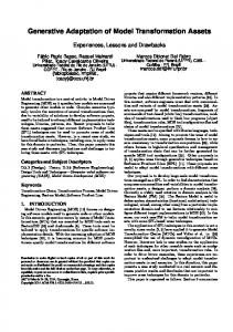
Model transformations can be classified in different ways [4, 12]. At a syntactic level, we can differentiate between those transformations where the source and target languages S and T are entirely disjoint, or where they overlap, or where one is a sub-language of the other. In the final case, transformations may be update-in-place, ie, they modify the elements of an existing model, rather than creating an entirely new model. Semantically, a transformation can be classified in terms of its role in a development process: Refinement A transformation that replaces source model elements by more complex target elements or structures to map an abstract model (such as a PIM) to a more specific version (such as a PSM). Code generation can be considered as a specific case. Abstraction A transformation that provides an abstraction of a model, such as the result of a query over the model. This is the opposite of a refinement. Quality improvement A transformation that remains at the same abstraction level, but that re-organises a model to achieve some quality goal (eg, removing duplicated attributes from a class diagram). Usually update-in-place. Re-expression A transformation that maps a model in one language into its equivalent in another language at the same level of abstraction, eg, migration transformations from one version of a language to another version. A small example of a re-expression transformation is a mapping between trees and graphs. Figure 1 shows the source and target metamodels of the transformation. The tree metamodel has the language constraint Asm1 that there are no non-trivial cycles in the parent relationship: t : Tree and t 6= t.parent implies t 6∈ t.parent + where r + is the non-reflexive transitive closure of r . Trees may be their own parent if they are the root node of a tree. In mapping from trees to graphs we also assume that the graph model is empty (Asm2): Edge = {} and Node = {}.
The graph metamodel has the constraint that edges must always connect different nodes (Ens1): e : Edge implies e.source 6= e.target and that edges are uniquely defined by their source and target, together (Ens2): e1 : Edge and e2 : Edge and e1.source = e2.source and e1.target = e2.target implies e1 = e2
Node name: String
Tree name: String {frozen, identity}
*
parent
{frozen, identity}
source
target
*
* Edge
Fig. 1. Tree to graph transformation metamodels
The identity constraint means that tree nodes must have unique names, and likewise for graph nodes. The transformation relates tree objects in the source model to node objects in the target model with the same name, and defines that there is an edge object in the target model for each non-trivial relationship from a tree node to its parent. 3.2
Conjunctive-implicative form
We consider first the case of unidirectional transformations τ , mapping from one language S to another (disjoint) language T , and with separate source and target models where the target model is empty at the start of the transformation and the source model is not changed by the transformation, ie, not update-inplace transformations. Such transformations include many cases of re-expression transformations such as model migrations, and refinements and abstractions. Let S1 , ..., Sn be the entities of S which are relevant to the transformation. Then one common specification pattern [28] is that Cons will have the general form of a conjunction of clauses, each of the form ∀ s : Si · SCondi,j implies ∃ t : Ti,j · TCondi,j and Posti,j where SCondi,j is a predicate over the source model elements only, Ti,j is some entity of T , TCondi,j is a condition in T elements only, eg., to specify explicit values for t’s attributes, and Posti,j refers to both t and s to specify t’s attributes
and possibly linked (dependent) objects in terms of s’s attributes and linked objects. SCond and TCond do not contain quantifiers, Post may contain ∃ quantifiers to specify creation/lookup of subordinate elements of t. If the t should be unique for a given s, the ∃1 quantifier may be alternatively used in the succedent of clauses. Additional ∀-quantifiers may be used at the outer level of the constraint, if quantification over groups of source model elements is necessary, instead of over single elements. For each Si there may be several clauses, and the SCondi,j should therefore be logically disjoint for distinct j if the corresponding right-hand sides of the implications are exclusive, in order that Cons is consistent. If some Si is a non-leaf class then its clauses can be duplicated for each of its subclasses, and the clauses for Si itself removed (for abstract non-leaf classes). We will therefore consider only leaf Si in this pattern. The pattern typically applies when S and T are similar in structure, for example in the UML to relational database mapping of [24, 18], the source structure of Package, Class, Attribute corresponds to the target structure of Schema, Table, Column. A simple example of the pattern is the specification of the tree to graph transformation by two global constraints: C1 “For each tree node in the source model there is a graph node in the target model with the same name”: ∀ t : Tree · ∃ n : Node · n.name = t.name C2 “For each non-trivial parent relationship in the source model, there is a unique edge representing the relationship in the target model”: ∀ t : Tree · t.parent 6= t implies ∃1 e : Edge · e.source = Node[t.name] and e.target = Node[t.parent.name] This illustrates a case where one source model element may produce two connected target model elements. The notation E [v ] denotes the E instance with primary key value v , if v is a single element, or the set of E instances with primary key values in v , if v is a collection. The constraints have a dual aspect: they express what conditions should be true at the completion of an entire transformation, but they can also be interpreted as the definitions of specific rules executed within the transformation. C 1 can be operationally interpreted as “For each tree node in the source model, create a graph node in the target model with the same name” and C 2 as “For each tree node with a distinct parent, create an edge linking the graph node corresponding to the tree node to the graph node corresponding to its parent, unless such an edge already exists.” We say that a predicate P is localised to elements s1 : Si1 , ..., sp : Sip in a language S if P only refers to expressions which are direct navigations from the si , or are constants from primitive and enumeration data types. Ideally the SCond and TCond expressions in a constraint are localised to s and t respectively, and Post to s, t.
Provided that the collection of TCondi,j conditions for each specific target entity Tl = Ti,j are logically exclusive, we can deduce reverse constraints/rules from Cons, which express that elements of T can only be created as a result of the application of one of the forward constraints/rules: each reverse rule has the form: ′ ∀ t : Ti,j · TCondi,j implies ∃ s : Si · SCondi,j and Posti,j ′ where Posti,j expresses the inverse of Posti,j . This predicate may not be explicit as a definition of s in terms of t, for example if Posti,j is
t.name = s.forename + “ ” + s.surname ′ there is no explicit inverse and Posti,j is the same as Posti,j . The reverse rules for the tree to graph specification are:
C3 “For each graph node in the target model there is a tree node in the source model with the same name”: ∀ g : Node · ∃ t : Tree · t.name = g.name C4 “For each edge in the target model, there is a unique non-trivial parent relationship in the source model, which the edge represents”: ∀ e : Edge · ∃1 t : Tree · t.parent 6= t and t = Tree[e.source.name] and t.parent = Tree[e.target.name] C 3 and C 4 are duals of C 1 and C 2. C 4 could be simplified to the equivalent constraint: ∀ e : Edge · Tree[e.source.name].parent = Tree[e.target.name] Examples of transformations which fit this pattern are the model migration transformation of UML 1.4 state machines to UML 2.2 activity diagrams [17], and the QVT-R implementation of the UML to relational database mapping, with persistent classes mapping to tables, packages to schemas, attributes to columns, etc [18]. Likewise for the re-expression transformation example of [31]. From the pattern we can deduce some general properties of this form of transformation: – Provided that the SCond predicates are localised to s, the TCond to t, and the Post are localised to s and t, all conditions can be effectively computed, and that the Post are explicit, the transformation is change-propagating for creation of new Si elements: the corresponding new Ti,j element(s) can be created and their feature values set according to which constraint has a true SCondi,j condition. – Likewise, if these conditions hold, and the Post ′ are localised, explicit and computable, we can change-propagate creation of new Ti,j elements using the reverse rules.
– Change-propagation of deletion of Si and Ti,j also follow under these assumptions, by considering the contrapositives of the reverse and forward rules, respectively. General propagation of attribute value changes however requires some tracing mechanism (such as identity attributes or attached stereotypes of target model elements) to connect specific source elements to the target elements whose values depend upon them. In particular, a change of attribute values of some s : Si may alter which SCondi,j holds true, implying that the T elements originally derived from s should be deleted and new elements created. The reverse rules of a transformation specification may provide only a partial inverse to the transformation, if it involves abstraction, because: – Not all entities of the source language may be used by the transformation, so that a source model with instances of such entities cannot be recreated by applying the reverse rules. Likewise if not all features of the Si are used by the transformation. – The forward transformation may not be injective, so that several different source models could produce the same target model. The reverse rules give a partial language-level interpretation χ : LS → LT , ′ provided the Posti,j are explicit and the SCondi,j are exclusive for distinct j : – χ({s : Si | SCondi,j }) is {t : Ti,j | TCondi,j } and therefore χ(Si ) is the union of the sets {t : Ti,j | TCondi,j } provided that the SCondi,j partition Si . ′ – Features att of Si which are explicitly set to expressions eatti,j in each Posti,j are interpreted by if self ∈ Ti,1 ∧ TCondi,1 [self /t] then tatti,1 [self /t] else ... else if self ∈ Ti,ni ∧ TCondi,ni [self /t] then tatti,ni [self /t] where tatti,j is the T object corresponding to eatti,j , if this is an object, otherwise it is eatti,j . χ is therefore partly determined by τ , although different variations on χ are possible. Essentially χ reconstructs a model of S from one of T , so that if an interpretation exists for each Si and feature of the source language this shows that T is at least as expressive as S , and that τ is reversible, because all information of the source model has been retained in the target: – If χ(Si ) exists for each entity Si of S , then this is an expression of LT which defines the set of objects of Ti,1 , ..., Ti,ni , etc corresponding to the elements of Si , ie, given an element t we can determine which Si it interprets.
– if χ(f ) exists for each data feature f of each Si of S , then this is an expression ′ built out of terms of T , and can be used to explicitly define f in Posti,j as t.χ(f ) or the S object corresponding to t.χ(f ). As the following counter-examples show, it is not possible to make further logical connections between the above general properties. – An example of a reversible transformation which has an interpretation but is not change propagating is given by S consisting of a single entity Entity with one (identity) attribute name : String, and the constraint name.size > 0. T also has a single entity Entity1 with one (identity) attribute name1 : String, and an inheritance relationship general /specific between Entity1 and itself (both ends are ∗). This has the language constraint specific = Entity1→select(e | name1 ≪ e.name1) (that is, the ‘subclasses’ of e1 are the entities whose name has e1’s name as a strict suffix (≪)), and the transformation is therefore specified by: ∀ e : Entity · ∃ e1 : Entity1 · e1.name1 = e.name and e1.specific = Entity1→select(e.name ≪ name1) The transformation is reversible by abstraction: simply discarding the specific/general association from the target model produces a model isomorphic to the source. The reverse implication is: ∀ e1 : Entity1 · ∃ e : Entity · e.name = e1.name1 The interpretation χ is also trivial, mapping Entity to Entity1 and name to name1. But the transformation is not change-propagating for creation, deletion or feature changes of the source model, since any such change could require examination of all the names of all instances in the target model, to compute the updated inheritance relation there. – A transformation which is change-propagating but has no interpretation and only a partial inverse, is given by S consisting of a single entity Entity with no attributes, T consisting of a single global integer attribute result : Integer , and Cons defined as: result = Entity→size() The first example is a refinement transformation, the second is an abstraction. The form of the Post predicates themselves will often be of one of the following kinds: – t.f = e where f is some feature of Ti,j and e an expression using feature values of s. – ∃ tsb : TSub · Posttsb and t.f = tsb to define a subpart of t. (Alternatively ∃ tsb : Set(TSub) can be used to select a set of subordinate elements, or ∃ tsb : Sequence(TSub) to select a sequence).
– Conjunctions of implications (Cond1 implies P1 ) and ... and (Condr implies Pr ) where the Pi are of the first two forms. A special case are equalities t.f = TSub[s.g.id 1] which select a single element of TSub or a set of elements, with primary key value(s) id 2 equal to s.g.id 1 (if this is a single value), or in the set s.g.id 1 (if it is a collection). The reversed form Post ′ is then s.g = SSub[t.f .id 2], if source model entity SSub is in 1-1 correspondence with TSub via the identities. 3.3
Special cases of conjunctive-implicative form
For each entity Si in the source language, there may be several different Ti,j entities on the right-hand side of implications in Cons, even with the same SCondi,j conditions. This may occur because the features of Si are being split or distributed between different target language entities, or because complex and separate structures are being generated in the target model from the same source data (akin to the Builder design pattern [7]). In these cases it is important to define in the separate target entities some key attribute or stereotype which records the fact of the semantic link between them (that they represent separate parts of the same source entity). This allows the definition of a semantic interpretation, and of a reverse relation. For example, consider the simple case where there is one source entity with attributes att1, att2, and key attribute id , and two target entities each with one of the attributes, but both having the key: ∀ s : S1 · ∃ t : T1 · t.id = s.id and t.att3 = s.att1 ∀ s : S1 · ∃ t : T2 · t.id = s.id and t.att4 = s.att2 The χ interpretation of S1 is {(t1, t2) : T1 × T2 | t1.id = t2.id }, and att1 can therefore be interpreted as att3 of the first projection on such pairs, and att2 as att4 of the second projection on such pairs. The reverse rules can be simply stated as: ∀ t : T1 · ∃ s : S1 · s.id = t.id and s.att1 = t.att3 ∀ t : T2 · ∃ s : S1 · s.id = t.id and s.att2 = t.att4 as with the general case of the conjunctive-implicative form. Without the identity attributes such definitions would not be possible. The reverse transformation illustrates another special form, where two source language entities are merged into a single target language entity. In this case both source entities are interpreted by the same target entity. The tree to graph transformation is another example of the special case, in which {t : Tree | t.parent = t} is interpreted by Node − Edge.source, the set of
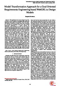
nodes which are not the source of any edge, whilst {t : Tree | t.parent 6= t} is interpreted by {(n, e) : Node × Edge | e.source = n} parent is interpreted by e.target in the second case. The one Si to multiple Tj case occurs in refinements, such as the generation of multiple J2EE elements (database tables, value objects, EJBs) from single UML classes. A large example carried out by one of the authors on a defence application was the mapping from data-flow diagrams to HOOD [6]. Data stores were mapped to classes, but processes with multiple flows were mapped to multiple operations on the different classes corresponding to the stores incident with the flows. Another variation on the conjunctive-implicative pattern occurs when the succedent of a constraint Cn both reads and writes to the same entity or feature: wr (Cn) ∩ (rd (Post) ∪ rd (TCond )) is non-empty, where wr (P ) is the write frame of a predicate P , and rd (P ) the read frame (Appendix B). Such constraints are said to be of type 2 (if the antecedent data and Si are not in wr (Cn)). Type 1 constraints have rd (Cn) ∩ wr (Cn) = {}. This means that the order of application of the constraint to instances may be significant, and that a single iteration through the source model elements may be insufficient to establish Post for all elements. A least-fixed point computation may be necessary instead, with iterations repeated until no further change takes place. An example is the derivation of the reachability relationship in a state machine (Figure 2). This is a refinement transformation, with the target language extending the source language, by the additional feature reaches. The constraint in this case is: ∀ t : Transition · {t.target} ∪ t.target.reaches ⊆ t.source.reaches Here the feature reaches is both read and written. A least fixed point does exist, if reaches is initialised to {}, since the reaches sets are monotonically increasing, and these sets are each bounded above by the set of all states. Therefore a terminating and confluent solution does exist for this specification. However the form of this solution is different to the simpler case where the sets of data written and read in a constraint are entirely disjoint (type 1 constraints). A measure Q : N on the source and target models is necessary to establish the termination and correctness of the implementation of type 2 constraints, and should be defined together with Cons. Q should be decreased by each application of a constraint, and Q = 0 at termination of the transformation. In this example, Q can be defined as: Σs:State (#states reachable from s) − #s.reaches
*
reaches
State name: String {identity}
source
1
*
1
*
target
*
Transition
Fig. 2. Metamodel for reachability computation
If for each particular starting state of the source and target models there is a unique possible modified state of the models (produced by applying the constraints) in which Q = 0, then the implementation is confluent. This is the case in this example. Likewise, a Q measure is necessary if Si ∈ wr (Cn) or wr (Cn) ∩ rd (SCond ) 6= {}, a constraint of type 3. An example of such a constraint is the derivation of the transitive closure of a graph [19]: ∀ e1, e2 : Edge · e1 6= e2 and e1.trg = e2.src implies ∃1 e3 : Edge · e3.src = e1.src and e3.trg = e2.trg For this, Q can be defined as the number of chains of edges in the original graph without an edge linking the start of the chain to its end. 3.4
Recursive forms
The conjunctive-implicative form presents the intended result of the transformation in an explicit form, but without any dependence upon a particular implementation strategy, thus facilitating validation and general comprehension. However in some cases the complexity of a transformation means that such a form is not possible, or it would be too far separated from the practical implementation of the transformation. A recursive form can be used instead, which defines the effect of the transformation as a recursive function (or set of recursive functions), each evaluation step of the function corresponds to the application of some transformation rule on a source model element, the recursion produces a final result when no further rule is applicable.
In effect the specification defines a function τ : ModelsS → ModelsT directly in terms of the concrete representations of the models as tuples (S1 , ..., f1 , ...), so that this approach is less abstract than the previous approach. We will assume that the source and target languages S and T are the same. Formally, the Cons predicate is defined as tmodel = τ (smodel @pre) where smodel is a tuple comprising the source model, and tmodel a tuple comprising the target model. τ is defined by a disjunction of constraints: (∃ s1 : S1 · SCond1 and ∃ t1 : Tj1 · τ (smodel ) = τ (smodel1 )) or ... (∃ sn : Sn · SCondn and ∃ tn : Tjn · τ (smodel ) = τ (smodeln )) or (not(∃ s1 : S1 · SCond1 ) and ... and not(∃ sn : Sn · SCondn ) and τ (smodel ) = smodel ) where the smodeli are updated versions of smodel using the selected domain elements si and generated elements ti . The left hand conditions ∃ si : Si · SCondi should be pairwise exclusive, to avoid inconsistencies. Alternatively their ordering could be used to define a priority on the rules/constraints. Quality-improvement transformations often follow this pattern, since they may be schematically specified by disjunctions of clauses (∃ e1 : S1 ; ...; en : Sn · SCond and ∃ f1 : Ti1 ; ...; fm : Tim · τ (smodel ) = τ (restr (smodel ))) where SCond is some condition identifying a lack of the desired quality in a model. For example, the existence of a class with two immediate ancestors, for a transformation that removes multiple inheritance. The restructuring restr depends on the ei and fj . A final clause (smodel satisfies all quality conditions and
τ (smodel ) = smodel )
terminates the recursion. Some quality measure Q : N should be definable, so that Q(restr (smodel )) < Q(smodel ) in each clause, and Q(smodel ) = 0 in the terminal cases. Q(smodel ) = Σc:Class
non root (c.generalization→size()
for the multiple-inheritance removal transformation.
− 1)
The constraint for the multiple-inheritance removal transformation could be written as follows in a simplified form of this style: ∃ c : Class; g : c.generalization · c.generalization→size() > 1 and g.general .allFeatures→size() = c.generalization.general →collect(allFeatures→size())→min() and ∃ a : Association · a.end 1 = c and a.end 2 = g.general and a.multiplicity1 = ONE and a.multiplicity2 = ZEROONE and g.isDeleted ()) meaning that τ (Class, Generalization, Association, Property, ownedAttribute, generalization, general , end 1, end 2, multiplicity1, multiplicity2, ...) is equal to τ of the updated model (Class, Generalization − {g}, Association ∪ {a}, Property, ownedAttribute, generalization − {c 7→ g}, general − {g 7→ g.general }, end 1 ∪ {a 7→ c}, end 2 ∪ {a 7→ g.general }, multiplicity1 ∪ {a 7→ ONE }, multiplicity2 ∪ {a 7→ ZEROONE }, ...) in the case that the antecedent holds for c and g (ie, that Q > 0 and g is some element of minimal semantic weight amongst the generalisations of c). The first representation of the constraint does not make sense as a property which must hold at the end state of a transformation, because g is both assumed to exist in the model and to be removed from the model. Only the formalised version using recursion to define τ can be interpreted logically. For convenience, however, the informal versions are used in UML-RSDS to define this form of transformation. It is difficult to establish change-propagation for recursive specifications, because a small change to the source model may affect an arbitrary number of evaluation steps of τ . Likewise, the construction of an interpretation involves consideration of each individual step. The specification may not identify a unique recursive function τ because the steps may not be confluent, even if the conditions of the cases are disjoint (this is the case for the multiple-inheritance removal transformation). However, inductive reasoning can be used to deduce properties which any solution to the recursion must satisfy, for example, that Class = Class@pre in this transformation, since no step modifies the set of classes. Other examples of the recursive pattern are the evaluation of OCL expressions using transformations in [22], the mapping of one representation of Lambda-expressions to another [8], slicing of state machines [16], and qualityimprovement transformations such as the removal of duplicated attributes in a class diagram, or the replacement of non-abstract superclasses by abstract classes. 3.5
Auxiliary metamodels
An additional specification pattern, which may be used with either the conjunctiveimplicative or recursive forms, is the use of an enhanced source or target meta-
model to express the specification. For example, in the state machine slicing transformation of [16], additional associations recording dependency sets of variables in each state, and the reachability relation between states, need to be added to the core state machine metamodel. In Figure 2 we have drawn the auxiliary metamodel element using dashed lines. Likewise for the lambda-calculus restructuring transformation [8], an additional association recording the set of bound variables in scope in each expression is required. Auxiliary metamodels are also used to implement tracing facilities, in transformation languages such as VIATRA [27] and Kermeta [10], the auxiliary entities and associations record information such as a history of rules applied and connections between target model elements and the source model elements they were derived from.
4
Implementation Patterns
Implementation of a model transformation may be carried out by the use of a special-purpose model transformation language such as ATL [9] or Kermeta [10], or by production of code in a general purpose language such as Java [15]. In either case, the implementation needs to be organised and structured in a modular manner, and ideally it should be possible to directly relate the implementation to the specification, expressed in the Cons predicate. We will use a small procedural language including assignment, conditionals, operation calls and loops to allow platform-independent imperative definitions of behaviour for transformation implementations (Figure 3). This language corresponds to a subset of UML structured activities.
0..1
StatKind sequence parallel choice
Behavior
Constraint invariant
{ordered} * statements
initialiser step 1 body 1
1
1 0..1
0..1
0..1
LoopStatement
Return Statement
Classifier
ifFalse 0..1 ifTrue 1
Statement
1 creates Instance Of 0..1
0..1
Conditional Statement
Sequence Statement
BasicStatement
kind: StatKind 0..1
0..1
0..1
* 0..1
0..1
BoundedLoop Statement
UnboundedLoop Statement 0..1
0..1
1 returns
0..1
test 1 1 test 0..1
Operation CallStatement
Assignment Statement
OclExpression
variant
0..1
0..1
*
1 left 1 right 1 target * actualParameters {ordered}
1
SkipStatement
left
Fig. 3. Statement metamodel
Creation Statement 0..1
1
calledOperation
Operation
4.1
Implementation strategies
We will consider three alternative strategies for implementation of a model transformation specification defined by a conjunctive-implicative or recursive pattern: – Change-propagation: the constraints are used directly to implement the transformation, by interpreting them in an operational form. If a change is made to the source model, any constraint whose lhs is made true by the change is applied, and the effects defined by its rhs are executed to modify the target model. – Recursive: the transformation is initiated by construction of instances of the topmost entities in the entity hierarchy of the target language T , such construction may require recursive construction of their components, etc. – Layered: the base elements (instances of the entities lowest in the entity hierarchy of T ) are constructed first, then elements that depend upon these are constructed, etc. It is possible to perform the layering from the top down, as in the Viatra version of the UML to relational database mapping [27], although this means that target model elements may be incomplete and invalid during the intermediate steps. Both the recursive and layered approaches make use of a partial order on the set of target language entities Tl [29], with instances of entities higher in the order being composed of (or being dependent upon) instances of entities below them in the order. In terms of the conjunctive-implicative form, this means that the constraints creating instances of Tk refer to an entity Tl (or a sub-or super-class of Tl ) in the TCond or Post predicates to define the Tk instances: Tk is then above Tl in the ordering. Formally, Tl < Tk if Tk ∈ wr (Cn) and Tl ∈ rd (Cn) for some constraint Cn. We will consider each strategy in detail in the following sections. 4.2
Change-propagation implementation
For transformations specified using the conjunctive-implicative form, it is in principle possible to interpret the constraints in an operational manner and to directly implement them using some constraint-driven development tool such as UML-RSDS [15], provided that the conditions for change-propagation hold: – The expressions SCond , TCond and Post are localised to s, t and s, t respectively, can be effectively computed, and Post is explicit. Lookup of objects by primary key value: Tk [e] can be considered localised and effective if e is. – There are 1-1 isomorphisms between source entity sets Si and corresponding S target entity sets j {t : Ti,j | TCondi,j }, induced by equal identity attribute values.
These conditions enable addition and attribute-change modifications to the source to be propagated to the target. The existential quantifier ∃1 t : Ti,j on the right hand side of a constraint can be interpreted as “if there does not exist an element t : Ti,j in the target model satisfying the conditions, create it and set its attributes using TCondi,j and Posti,j ” if Ti,j is concrete. This interpretation is also used for ∃ t : Ti,j if Ti,j has an identity attribute – creation of two Ti,j objects with the same value for this attribute would violate the constraints of T . We call this the unique instantiation pattern. QVT has a similar mechanism, check-before-enforce, to reuse target model elements that satisfy a relation, in preference to recreating new elements [23]. Otherwise the ∃ t : Ti,j quantifier does not check before creating a t instance for concrete Ti,j . 4.3
Recursive implementation
This strategy is typically used in transformation languages such as QVT and ATL, via explicit or implicit invocation of relations from other relations (the where clause in QVT). For example, the QVT version of the UML to relational database mapping initiates processing by mapping packages to schemas, then maps the classes of individual packages to relational tables, in turn this involves the mapping of attributes to columns, and finally of UML types to database types [24]. Such a strategy requires that a strict hierarchy exists between the target language entities, ie, there should be a partial order E1 < E2 meaning that E2 is composed of E1 elements (directly or indirectly). In this example, Column < Table < Schema At each stage the superordinate target entity instances are passed down to the rules defining the subordinate entity instances, for example in our pseudocode notation we could express this transformation as follows: mapPackageToSchema(p : Package) : Schema (result.name := p.name; for c : p.classes do mapClassToTable(c, result); return result) mapClassToTable(c : Class, s : Schema) (t : Table; t.name := c.name; t.schema := s; for a : c.allAttribute do mapAttributeToColumn(a, t)) mapAttributeToColumn(a : Attribute, t : Table) (cl : Column; cl .name := a.name; cl .table := t; cl .type := typeConvert(a.type))
This approach could be termed the recursive descent pattern. This is effective if the object hierarchy in T does not involve sharing of objects, so that the recursive descent of the corresponding S hierarchy can create T structures depending only on subordinate and superordinate objects in the object hierarchy. Here, although attributes may be in common between some source classes, distinct copies of the corresponding columns are required in the target model. If instead, target elements need to be shared, some lookup mechanism is required to match source model elements and target model elements generated from them (this lookup is performed implicitly in ATL). Where an entity depends upon itself (as for trees in the tree to graph example), recursion down the object structure (using the inverse relation to parent in this case) can be used if this structure is hierarchical. A technique for synthesising a recursive implementation from a declarative specification using constructive proofs based on partial orderings of metamodel entities is given in [29]. 4.4
Layered implementation
The layered approach has the advantage that it can be carried out in a phased manner: by the sequential composition of separate sub-transformations, each responsible for adding one more layer of structure to the target model, assuming that previous phases have already constructed the lower layers. This implementation of the layered approach could be called the phased creation pattern. This strategy reduces the complexity of the transformation compared to the recursive approach, and increases the modularity, by reducing calling dependencies, and makes verification more simple, in particular, proof of termination. However it may be inefficient, because it requires the lookup of constructed elements of a lower level, each time a new element of a higher level is created. Such a lookup may typically be done by a key-based search, or by using an explicit transformation trace facility, as in Kermeta [10] and VIATRA [27]. The UML-RSDS tools efficiently implement searches for the set of elements TSub[sexp.id 1] of a target type TSub with primary key values in sexp.id 1 by maintaining a map from the primary keys of TSub objects to the objects – this could be termed the object indexing pattern. In some cases no clear hierarchy of target language entities exists, for example, there may be mutally dependent entities T1 and T2 in the target model. In such a case a phased approach can first construct all the T1 and T2 instances, in any order, then establish the links (in both directions) between them. For example, if T1 has a feature att : T2 and T2 has a feature role : Set(T1 ) and these are not mutual inverses. This approach can also be used if a target entity Tj depends on itself, or we can use some hierarchical structure for the set of Tj instances in order to implement layered construction of Tj objects. Phased implementation can be used to separate a phase of object construction from a ‘cleanup’ phase where unwanted objects are deleted, the construction and cleanup pattern.
A hybrid approach is possible, whereby the layered approach is primarily used, but recursive construction of exclusively-owned subparts TSub of an entity T is used. Such subparts may typically be entities which do not have a separate identity attribute of their own, so lookup by identity cannot be used for them. For a phased implementation, the form of the specification can be used to define the individual transformation rules. If Cons is a conjunction of constraints Ci of the form ∀ s : Si · SCond implies ∃ t : Tj · TCond and Post then each constraint may be mapped individually into a phase Pi which implements it, provided that there are no circularities in the data dependency relationship between constraints. We define Ci < Cj if wr (Ci ) ∩ rd (Cj ) 6= {} This should be a partial order, and should imply that i < j . The phases can be executed in any order that is consistent with this data dependency ordering Ci < Cj , including concurrent execution if the phases are not related by data dependency. Pj will establish Cj at its termination, under the assumption that Ci holds for each Ci < Cj , ie, that each corresponding Pi has been completed and that Ci has not been invalidated by succeeding phases. This can be ensured if the write frames of distinct constraints are disjoint. If a group of constraints are mutually data dependent, then they must be implemented by a single phase. In the simple case where a constraint satisfies the non-interference condition: wr (Ci ) ∩ rd (Ci ) = {} the (type 1) constraint can be implemented by a loop for s : Si do s.opi () where in Si we include an operation of the form: opi () post: SCond [self /s]
implies
∃ t : Tj · TCond and Post[self /s]
We refer to this strategy as constraint implementation approach 1. The proof of correctness of this strategy uses the property that the inference rule: from v : s ⇒ [acts(v )]P (v ) derive [for v : s do acts(v )](∀ v : s@pre · P (v )) is valid for such iterations, provided that one execution of acts does not affect another: the precondition of each acts(v ) has the same value at the start of
acts(v ) as at the start of the loop, and if acts(v ) establishes P (v ) at its termination, P (v ) remains true at the end of the loop [15]. Confluence also follows if the updates of written data in different executions of the loop body are independent of the order of the executions. For the tree to graph example, C 1 < C 2, so the phase creating nodes must precede that creating edges. Phase 1 uses the operation mapTreeToNode() post: ∃ n : Node · n.name = name of Tree to map a tree to a node. Since the updates to Node and Node :: name are independent for distinct n, the implementation will be confluent. The activity for this phase is a simple unordered iteration over all tree elements: for t : Tree do t.mapTreeToNode() This iteration executes mapTreeToNode() exactly once for each t in Tree at the start of the loop execution. It can also be denoted by Tree.mapTreeToNode(). Phase 2 creates edges, assuming that phase 1 has been completed. For phase2 the operation is: mapTreeToEdge() post: self 6= parent
implies ∃1 e : Edge · e.source = Node[name] and e.target = Node[parent.name]
this is also iterated over Tree, and is also confluent. A more complex implementation strategy is required if the non-interference condition does not hold. Consider a constraint Ci : ∀ s : Si · SCond implies ∃ t : Tj · TCond and Post where this is the only Si constraint. In the case where wr (Ci ) ∩ (rd (Post) ∪ rd (TCond )) is non-empty but the other conditions of non-interference still hold (a type 2 constraint), an iteration of the form: running := true; while (running) do (running := false; for s : Si do if SCond then if Succ then skip else (s.op(); running := true) else skip)
can be used, where Succ is ∃ t : Tj · TCond and Post and op() is defined as: op() post: Succ[self /s] (We refer to this strategy as constraint implementation approach number 2). The conditional test of Succ can be omitted if it is known that SCond ⇒ not(Succ). If the updates to the written data are monotone and bounded (eg, as in the case of the inclusion operator ⊆ for the reachability computation example), then the iteration terminates and computes the least fixed point. A measure Q : N can be used to prove termination, a suitable measure in this case is the sum Σs:State (#states reachable from s) − #s.reaches. Q is decreased by each application of op and is never increased. Q is also necessary to prove correctness: while there remain s : Si with SCond true but Succ false, then Q > 0 and the iteration will apply op to such an s. At termination the constraint therefore holds true, and Q = 0. Confluence also follows if Q = 0 is only possible in one unique state of the source and target models which can be reached from the initial state by applying the constraint. For the reachability computation, the inner loop iterates: if { t.target } ∪ t.target.reaches ⊆ source.reaches then skip else (t.op(); running := true) If the other conditions of non-interference fail (a type 3 constraint), then the application of a constraint to one element may change the elements to which the constraint may subsequently be applied to, so that a fixed for -loop iteration over these elements cannot be used. Instead, a schematic iteration of the form: while some source element s satisfies a constraint lhs do select such an s and apply the constraint can be used. This can be explicitly coded as: running := true; while running do running := search() where: search() : Boolean (for s : Si do if SCond then if Succ then skip else (s.op(); return true)); return false
and where op applies the constraint succedent. We call this approach 3, iteration of a search-and-return loop. The conditional test of Succ can be omitted if it is known that SCond ⇒ not(Succ). As in approach 2, a Q measure is needed to prove termination and correctness. search returns false exactly when Q = 0. Again, confluence can be deduced from uniqueness of the termination state. For the multiple-inheritance removal transformation, the search operation is: (for c : Class do for g : c.generalization do if c.generalization→size() > 1 and g.general .allFeatures→size() = c.generalization.general →collect(allFeatures→size())→min() then (c.op(g); return true)); return false The operation is applied repeatedly to remove multiple inheritances from the model, until no case remains (ie, when Q = 0). Here the termination states are not unique and confluence fails. For quality-improvement transformations the Q metric can be used to select constraints: the constraint application which maximally reduces this measure can be chosen if several are possible. In summary, we have identified the following implementation patterns: – Unique instantiation: before creating an instance to satisfy ∃1 t : TType · TPred , search to see if one already exists, and use this if so. This is related to the Singleton pattern [7] and may use Object indexing. – Object indexing: to find collections TType[ids] of TType elements with a given set ids of primary key values, maintain a map from primary keys to TType elements. – Recursive descent: recursively map subcomponents of a source model element as part of the mapping operation of the element, passing down the target object(s) in order to link subordinate target elements to it/them. – Phased creation: before creating an instance of an entity T1 , create all instances of entities T2 hierarchically below T1 , which are mapped to by the transformation. In the case of mutually dependent entities, create all objects of the entities before setting the links between them. – Construction and cleanup: separate construction of new elements from the removal of deleted elements, placing these processes in successive phases. The Builder and Abstract Factory patterns are also directly relevant to pattern implementation, in cases where complex platform-specific structures of elements must be constructed from semantic information in a platform-independent model, such as the synthesis of J2EE systems from UML specifications.
5
Formalisation of model transformation design
The process of deriving designs for a model transformation from its specification can be formalised and expressed itself as a (meta) model transformation at the
M2 level. The key parts of the source and target languages are given in Figure 4, the statement language is defined in Figure 3. Transformations are considered to be particular use cases of a system. Use cases may have pre and postconditions (Ens and Cons constraint sets for transformations) and invariant properties (Pres for transformations).
Extend
extend 1 * extension
0..1
1
* * {ordered} extension Location 1..* Extension Point
ordered Postconditions UseCase
extended Case 1
0..1
Constraint
postcondition * {ordered} primaryClass() : Class body() : OclExpression * primaryVar() : String rd() : Set(String) wr() : Set(String) secondaryVars() : Sequence 0..1
0..1 classifierBehavior
*
Behavior
1 implementedBy Class
*
0..1
Operation
owned Operation
0..1
Fig. 4. Transformation specification metamodel
We have extended the UML metamodel with auxiliary associations orderedPostconditions and implementedBy, and auxiliary query operations to return the read and write frame of constraints, and to return the main quantified class and variable, secondary quantified variables, and the quantified body of the constraint. Individual constraints Cn: ∀ s : Si · SCond implies ∃ t : Tj · TCond and Post are examined to identify which implementation strategy can be used to derive their design. This depends upon the features and objects read and written within the constraint (Table 1). The set of constraints are also examined to determine the dependency relation < between constraints. It is assumed that the constraints are consistent, and that the specifier has ordered the constraints so that C1 precedes C2 if rd (C2 )∩wr (C1 ) is non-empty. If a group of constraints are mutually data-dependent, then they are mapped into a single phase, implemented using approach 2 or 3. In the case that there are two mutually dependent constraints with outer quantifier ∀ s : Si , approach 2 has the form running := true; while (running) do (running := false; for s : Si do loop) where loop is the code: if SCond 1 then
Constraint properties Implementation choice Type 1 No interference between Approach 1: single for loop constraint different applications of constraint, and no for s : Si do s.op() change to Si or rd (SCond ): wr (Cn) ∩ rd (Cn) = {}. Type 2 Interference between Approach 2: while constraint different applications of iteration of for loop. constraint, but no update of Si or rd (SCond ) Q measure needed within constraint: Si 6∈ wr (Cn), for termination and wr (Cn) ∩ rd (SCond ) = {} correctness proof Type 3 Update of Approach 3: while iteration of constraint Si or rd (SCond ) search-and-return for loop within constraint. Q measure needed Si ∈ wr (Cn), or for termination and wr (Cn) ∩ rd (SCond ) 6= {} correctness proof Table 1. Design choices for constraints
if Succ1 then else (s.op1(); if SCond 2 then if Succ2 then else (s.op2();
skip running := true); skip running := true)
op1 implements the succedent of the first constraint, and op2 that of the second. Similar extensions can be made for approach 3, and for approach 2 and 3 with distinct source entities for the outer quantifier. The generated code of each phase can then be combined in an overall sequence statement. This meta-transformation itself follows the conjunctive implicative pattern. For example, the constraint defining the construction of simple iterations for type 1 constraints ∀ s : Si · SCond implies ∃ t : Tj · TCond and Post is: ∀ u : UseCase; c : u.orderedPostconditions · rd (c) ∩ wr (c) = {} and secondaryVars(c) = Sequence{} implies ∃ d : Operation · d .name = u.name + c.name and d : primaryClass(c).ownedOperation and body(c).substitute(“self ”, primaryVar (c)) : d .postcondition and ∃ stat : OperationCallStatement · stat.calledOperation = d and stat.target = primaryClass(c).allInstancesExp() and c.implementedBy = stat cl .allInstancesExp() returns the OCL CallExp representing Si .allInstances(), if cl represents Si .
In a final phase, all constraint implementations are gathered into a sequence statement: ∀ u : UseCase · ∃ stat : SequenceStatement · stat.statements = u.orderedPostconditions.implementedBy and stat : u.classifierBehavior Use cases are a subclass of BehavioredClassifier in UML, so they have a classifierBehavior . We use this to define the overall activity which implements the use case. The transformation is an update-in-place transformation, in which all the constraints are of the first kind in Table 1. In the UML-RSDS tools it is implemented in a change-propagating manner: when a new constraint is added to a use case, the implementing operations and activities of the use case are automatically updated. We intend to also support the generation of checking transformations from use case preconditions (Asm constraints) and inverse transformations from the Cons constraints of invertible transformations. The UML-RSDS tools, together with examples of transformation specification and implementation, are available at: http : //www .dcs.kcl .ac.uk /staff /kcl / uml 2web/.
6
Related Work
In [3], specifications of the conjunctive-implicative form are derived from model transformation implementations in triple graph grammars and QVT, in order to analyse properties of the transformations, such as definedness and determinacy. This form of specification is therefore implicitly present in QVT and other transformation languages, and we consider that it is preferable for such logical specifications to be defined prior to detailed coding of the transformation rules, in order to identify possible errors at an earlier development stage. In [28] the concept of the conjunctive-implicitive form was introduced to support the automated derivation of transformation implementations from specifications written in a constructive type theory. A single undecomposed constraint of the ∀ ⇒ ∃ form defines the entire transformation, and the constructive proof of this formula produces a function which implements the transformation. In [29] the conjunctive-implicative form is used as the basis of model transformation specifications in constructive type theory, with the ∃ x .P quantifier interpreted as an obligation to construct a witness element x satisfying P . A partial ordering of entities is used to successively construct such witnesses. In this paper we show how this approach may be carried out in the context of first order logic, with systematic strategies and patterns used to derive transformation implementations from transformation specifications, based on the detailed structure of the specifications. The correctness of the strategies and patterns are already established and do not need to be re-proved for each transformation, although side conditions (such as the data-dependency conditions and existence of a suitable Q measure) need to be established.
In [1], a transformation specification pattern is introduced, Transformation parameters, to represent the case where some auxiliary information is needed to configure a transformation. This could be considered as a special case of the auxiliary metamodel pattern. An implementation pattern Multiple matching is also defined, to simulate rules with multiple element matching on their antecedent side, using single element matching. We also use this pattern, via the use of multiple ∀ quantifiers in specifications and multiple for loops at the design level to select groups of elements. Our work extends previous work on model transformation patterns by combining patterns into an overall process for developing model transformation designs and implementations from their specifications.
7
Summary
We have described three specification patterns: the conjunctive-implicative and recursive forms of specification constraints and the auxiliary metamodel pattern, and five implementation patterns. We have described how the form of specification constraints can be used to deduce global properties of a transformation, and can be used to construct an implementation. Quality metrics could also be based on the patterns, for example measures of the degree of locality of data accesses in the specification of a model transformation would be relevant to the efficiency and modularity of the transformation.
Acknowledgement The work presented here was carried out in the EPSRC HoRTMoDA project at King’s College London.
References 1. J. Bezivin, F. Jouault, J. Palies, Towards Model Transformation Design Patterns, ATLAS group, University of Nantes, 2003. 2. J. Bezivin, F. Buttner, M. Gogolla, F. Jouault, I. Kurtev, A. Lindow, Model Transformations? Transformation Models!. 3. J. Cabot, R. Clariso, E. Guerra, J. De Lara, Verification and Validation of Declarative Model-to-Model Transformations Through Invariants, Journal of Systems and Software, preprint, 2009. 4. K. Czarnecki, S. Helsen, Classification of Model Transformation Approaches, OOPSLA 03 workshop on Generative Techniques in the context of Model-Driven Architecture, OOPSLA 2003. 5. Eclipse organisation, EMF Ecore specification, http://www.eclipse.org/emf, 2011. 6. ESA, HOOD Reference Manual R4, http://www.esa.int, 2011. 7. E. Gamma, R. Helm, R. Johnson, J. Vlissides, Design Patterns: Elements of Reusable Object-Oriented Software, Addison-Wesley, 1994. 8. P. Van Gorp, S. Mazanek, A. Rensink, Live Challenge Problem, TTC 2010, Malaga, July 2010.
9. F. Jouault, I. Kurtev, Transforming Models with ATL, in MoDELS 2005, LNCS Vol. 3844, pp. 128–138, Springer-Verlag, 2006. 10. Kermeta, http://www.kermeta.org, 2010. 11. S. Kolahdouz-Rahimi, K. Lano, A Model-based Development Approach for Model Transformations, FSEN 2011, Iran, 2011. 12. T. Mens, K. Czarnecki, P. Van Gorp, A Taxonomy of Model Transformations, Dagstuhl Seminar Proceedings 04101, 2005. 13. K. Lano (ed.), UML 2 Semantics and Applications, Wiley, New York, 400 pages, 2009. 14. K. Lano, A Compositional Semantics of UML-RSDS, SoSyM, 8(1): 85–116, 2009. 15. K. Lano, S. Kolahdouz-Rahimi, Specification and Verification of Model Transformations using UML-RSDS, IFM 2010, LNCS vol. 6396, pp. 199–214, 2010. 16. K. Lano, S. Kolahdouz-Rahimi, Slicing of UML models using Model Transformations, MODELS 2010, LNCS vol. 6395, pp. 228–242, 2010. 17. K. Lano, S. Kolahdouz-Rahimi, Migration case study using UML-RSDS, TTC 2010, Malaga, Spain, July 2010. 18. K. Lano, S. Kolahdouz-Rahimi, Model-driven development of model transformations, ICMT 2011, June 2011. 19. K. Lano, S. Kolahdouz-Rahimi, Specification of the “Hello World” case study, submitted to TTC 2011. 20. K. Lano, S. Kolahdouz-Rahimi, Specification of the GMF migration case study, submitted to TTC 2011. 21. K. Lano, Class diagram rationalisation case study, Dept. of Informatics, King’s College London, 2011. 22. S. Markovic, T. Baar, Semantics of OCL Specified with QVT, Software and Systems Modelling, vol. 7, no. 4, October 2008. 23. OMG, Query/View/Transformation Specification, ptc/05-11-01, 2005. 24. OMG, Query/View/Transformation Specification, annex A, 2010. 25. OMG, Model-Driven Architecture, http://www.omg.org/mda/, 2004. 26. OMG, Meta Object Facility (MOF) Core Specification, OMG document formal/0601-01, 2006. 27. OptXware, The Viatra-I Model Transformation Framework Users Guide, 2010. 28. I. Poernomo, Proofs as model transformations, ICMT 2008. 29. I. Poernomo, J. Terrell, Correct-by-construction Model Transformations from Spanning tree specifications in Coq, ICFEM 2010. 30. P. Stevens, Bidirectional model transformations in QVT, SoSyM vol. 9, no. 1, 2010. 31. L. Tratt, Model transformations and tool integration, SoSym, 2005.
A
Formal statement of patterns
In this section we define the transformation patterns using the standard GoF pattern documentation format [7].
A.1
Conjunctive implicative form
Synopsis To specify the effect of a transformation in a declarative manner, as a global pre/post predicate, consisting of a conjunction of constraints with a ∀ ⇒ ∃ structure.
Forces Useful whenever a platform-independent specification of a transformation is suitable. The conjunctive-implicative form can be used to analyse the semantics of a transformation, and also to construct an implementation. Solution The Cons predicate should be split into separate conjuncts each relating one (or a group) of source model elements to one (or a group) of target model elements: ∀ s : Si · SCondi,j implies ∃ t : Ti,j · TCondi,j and Posti,j where the Si are source entities, the Ti,j are target model entities, SCondi,j is a predicate on s (identifying which elements the constraint should apply to), and Posti,j defines t in terms of s. For Cons specifications including type 2 or type 3 constraints, suitable Q measures are needed to establish termination, confluence and correctness of the derived transformation implementation.
Consequences The Ens and Pres properties should be provable directly from the constraints: typically by using the Cons constraints that relate the particular entities used in specific Ens or Pres constraints.
Implementation Either by the change-propagation, layered or recursive implementation strategies.
Code examples A large example of this approach for a migration transformation is in [17]. The UML to relational mapping is also specified in this style in [18]. In this paper we have described the tree to graph transformation in detail. In this case Ens1 follows from C 1, C 2 and the uniqueness of name on trees and nodes, Ens2 follows from C 2.
A.2
Recursive form
Synopsis To specify the effect of a transformation in a declarative manner, as a global pre/post predicate, using a recursive definition of the transformation relation.
Forces Useful whenever a platform-independent specification of a transformation is required, and the conjunctive-implicative form is not applicable, because the poststate of the transformation cannot be directly characterised or simply related to the pre-state. Solution The Cons predicate is defined by an equation such as tmodel = τ (smodel @pre) or more generally as (smodel , tmodel ) = τ (smodel @pre, tmodel @pre) where smodel represents the source model and tmodel the target model, and τ is a recursive function defined by a disjunction of clauses ∃ s : Si · SCondi,j and ∃ t : Ti,j · TCondi,j and Posti,j
where the Si are source entities, the Ti,j are target model entities, SCondi,j is a predicate on s (identifying which elements the constraint should apply to), and Posti,j defines the mapping τ (smodel , tmodel ) in terms of smodel , tmodel , s, t and other mapping forms τ (smodel ′ , tmodel ′ ) for some modified models smodel ′ , tmodel ′ derived from smodel , tmodel . The ∃ s : Si · SCondi,j conditions should be pairwise exclusive, or the ordering of the constraints used to define a priority ordering of tests. There should exist a measure Q : N on the state of a model, such that Q is decreased on each step of the recursion, and with Q = 0 being the termination condition of the recursion. A default case with conclusion τ (smodel , tmodel ) = (smodel , tmodel ) applies in this case. Q is an abstract measure of the time complexity of the transformation, the maximum number of steps needed to complete the transformation on a particular model. For quality-improvement transformations it can also be regarded as a measure of the (lack of) quality of a model.
Consequences The proof of Ens and Pres properties from Cons is more indirect for this style of specification, typically requiring induction using the recursive definitions. Implementation The constraints can be used to define a recursive operation that satisfies the specification, or an equivalent iterative form. The constraints can also be used to define pattern-matching rules in transformation languages such as ATL or QVT.
Code examples Many computer science problems can be expressed in this form, such as sorting, searching and scheduling. For example, the sorting of a list s of integers ordered by < is: (∃ i, j : 1 . . s→size() · i < j and s(j ) < s(i) and τ (s) = τ (s ⊕ {i 7→ s(j ), j 7→ s(i)})) or ((∀ i, j : 1 . . s→size() · i < j implies s(i) ≤ s(j )) and τ (s) = s) The quality measure Q(s) is the number of disorderings in s, ie, the number of pairs i, j of indexes satisfying the antecedent of the first constraint. The recursion terminates when this reaches 0: Q(s) = 0 implies τ (s) = s Q(s) in the worst case is of order n 2 , where n is the size of s. An iterative implementation of this problem in Java could be: boolean running = true; while (running) { running = rule1(s); } where: public static boolean rule1(int[] s) { for (int i = 0; i < s.size(); i++) { for (int j = i+1; j < s.size(); j++) { if (s[j] < s[i]) { int temp = s[i]; s[i] = s[j];
s[j] = temp; return true; } } } return false; } We use the implementation approach 3, as for type 3 constraints, to implement recursive specifications in Java.
A.3
Auxiliary metamodel
Synopsis The introduction of a metamodel for auxiliary data, neither part of the source or target language, used in a model transformation.
Forces Useful whenever auxiliary data needs to be used in a transformation: such data may simplify the transformation definition, and may permit a more convenient use of the transformation, eg., by supporting decomposition into sub-transformations. A typical case is a query transformation which counts the number of instances of a complex structure in the source model: explicitly representing these instances as instances of a new (auxiliary) entity may simplify the transformation. Tracing can also be carried out by using auxiliary data to record the history of transformation steps within a transformation.
Solution Define the auxiliary metamodel as a set of (meta) attributes, associations, entities and generalisations extending the source and/or target metamodels. These elements may be used in the succedents of Cons constraints (to define how the auxiliary data is derived from source model data) or in antecedents (to define how target model data is derived from the auxiliary data).
Consequences It may be necessary to remove auxiliary data from a target model, if this model must conform to a specific target language at termination of the transformation. A final phase in the transformation could be defined to delete the data (cf. the construction and cleanup pattern).
Code example An example is a transformation which returns the number of cycles of three distinct nodes in a graph. This problem can be elegantly solved by extending the basic graph metamodel by defining an auxiliary entity ThreeCycle which records the 3-cycles in the graph (Figure 5). The auxiliary language elements are shown with dashed lines. The specification Cons of this transformation then defines how unique elements of ThreeCycle are derived from the graph, and returns the cardinality of this type at the end state of the transformation: (C 1) : ∀ g : Graph · ∀ e1 : g.edges; e2 : g.edges; e3 : g.edges · e1.trg = e2.src and e2.trg = e3.src and e3.trg = e1.src and (e1.src ∪ e2.src ∪ e3.src)→size() = 3 implies ∃1 tc : ThreeCycle · tc.elements = (e1.src ∪ e2.src ∪ e3.src) and tc : g.cycles
edges *
Edge
*
num: Integer 1
*
trg src 0..1 0..1 *
IntResult
Graph 1
1
* cycles nodes ThreeCycle
Node name : String elements
*
*
Fig. 5. Extended graph metamodel
(C 2) : ∀ g : Graph · ∃ r : IntResult · r .num = g.cycles→size() The alternative to introducing the intermediate entity would be a more complex definition of the constraints, involving the construction of sets of sets using OCL collect.
Related patterns This pattern extends the conjunctive-implicative and recursive form patterns, by allowing constraints to refer to data which is neither part of the source or target languages. A.4
Construction and cleanup
Synopsis To simplify a transformation by separating rules which construct model elements from those which delete elements. Forces Useful when a transformation both creates and deletes elements of entities, resulting in complex specifications. Solution Separate the creation phase and deletion phase into separate constraints, usually the creation (construction phase) will precede the deletion (cleanup). These can be implemented as separate transformations, each with a simpler specification and coding than the single transformation. Consequences The pattern leads to the production of intermediate models (between construction and deletion) which may be invalid as models of either the source or target languages. It may be necessary to form an enlarged language for such models. Code examples An example is migration transformations where there are common entities between the source and target languages [20]. A first phase copies/adapts any necessary data from the old version (source) entities which are absent in the new version (target) language, and creates data for new entities, then a second phase removes all elements of the model which are not in the target language. The intermediate model is a model of a union language of the source and target languages.
Another example are complex update-in-place transformations, such as the removal of duplicated attributes [21]. A rule (in the recursive style) which moves attributes duplicated in all direct subclasses of a class up to the class, could be: ∀ c : Class · c.specialization→size() > 1 implies ∀ a : c.specialization.specific.ownedAttribute · c.specialization.specific→forAll ( ownedAttribute→exists(name = a.name and type = a.type)) implies ∃ p : Property · p.name = a.name and p.type = a.type and p : c.ownedAttribute and c.specialization.specific→forAll (a.name 6∈ ownedAttribute.name) This both creates a new attribute of the superclass with the duplicated name and type, and removes the attribute copies from the subclasses. Instead, the constraint can be rewritten to only create p, and a separate constraint defined to subsequently remove the copies: ∀ c : Class; p : c.allAttribute; c1 : c.specialization.specific · c1.ownedAttribute→select(name = p.name)→isDeleted () e→exists(x | P ) is OCL syntax for ∃ x : e · P , e→forAll (x | P ) is OCL syntax for ∀ x : e · P. Another implementation strategy for this pattern is to explicitly mark the unwanted elements for deletion in the first phase, and then to carry out the deletion of marked elements in the second phase. In this example an additional flag attribute of Property could be used to indicate which subclass properties should be removed. A similar approach can be applied to the transformation to remove multiple inheritance: a first phase could mark the generalisations to be removed, a second phase could introduce the replacement associations, and a third deletes the marked generalisations.
A.5
Unique instantiation
Synopsis To avoid duplicate creation of objects in the target model, a check is made that an object satisfying specified properties does not already exist, before such an object is created. Forces Required when duplicated copies of objects in the target model are forbidden, either explicitly by use of the ∃1 t : Tj · Post quantifier, or implicitly by the fact that Tj possesses an identifier (primary key) attribute.
Solution To implement a specification ∃1 t : Tj · Post for a concrete class Tj , test if
∃ t : Tj · Post is already true. If so, take no action, otherwise, create a new instance t of Tj and establish Post for this t. In the case of a specification ∃ t : Tj · t.id = x and Post where id is a primary key attribute, check if a Tj object with this id value already exists: x ∈ Tj .id and if so, use the object (Tj [x ]) to establish Post.
Consequences The pattern ensures the correct implementation of the constraint. It can be used when we wish to share one subordinate object between several referring objects: the subordinate object is created only once, and is subsequently shared by the referrers.
Implementation The executable ‘update form’ in Java of ∃1 t : Tj · Post for a concrete class Tj is:
if (qf ) { } else { uf } where qf is the query form of ∃ t : Tj · Post, and uf is its update form. The update form of ∃ t : Tj · t.id = x and Post for a class Tj with primary key id is: Tj t; if (qf ) { t = Controller.inst().getTjByPK(x’); } else { uf ; } Post∗ where qf is the query form of x : Tj .id , x ′ the query form of x , Post∗ the update form of Post, and uf creates a new instance t of Tj with t.id = x .
Code example Here is sample code, created to check the uniqueness of a ThreeCycle in a graph, corresponding to the succedent of constraint C 1 above: if (Set.exists_0(Controller.inst().threecycles, this, e1, e2, e3)) {} else { ThreeCycle tc = new ThreeCycle(); Controller.inst().addThreeCycle(tc); Controller.inst().addcycles(this,tc); Controller.inst().setelements(tc,Set.union(e1.getsrc(), Set.union(e2.getsrc(),e3.getsrc()))); } where the exists 0 query operation tests if there is already a three cycle with the given elements in this.cycles. The ‘check before enforce’ matching semantics for QVT rules is another example of the pattern.
Related patterns Object indexing can be used to efficiently obtain an object with a given primary key value in the second varient of the pattern.
A.6
Object indexing
Synopsis All objects of a class are indexed by a unique key value, to permit efficient lookup of objects by their key.
Forces Required when frequent access is needed to objects or sets of objects based upon some unique identifier attribute (a primary key).
Solution Maintain an index map data structure cmap of type IndType → C , where C is the class to be indexed, and IndType the type of its primary key. Access to a C object with key value v is then obtained by applying cmap to v : cmap.get(v ).
Consequences The key value of an object should not be changed after its creation: any such change will require an update of cmap, including a check that the new key value is not already used in another object.
Implementation When a new C object c is created, add c.ind 7→ c to cmap. When c is deleted, remove this pair from cmap. To look up C objects by their id, apply cmap. An alternative strategy to look up target model elements is to use an explicit transformation trace facility, as in Kermeta [10] and VIATRA [27]. Code example Here is sample code, as generated by the UML-RSDS tools for an entity Person with primary key pid : String. In the Controller class representing the system, there are attributes List persons = new Vector(); // of Person Map personindex = new HashMap(); // String -> Person representing the set of existing Person objects, and the indexing map. This class has operations: public void addPerson(Person p) { persons.add(p); personindex.put(p.getpid(),p): } public void removePerson(Person p) { persons.remove(p); personindex.remove(p.getpid()): } public Person getPersonByPK(String pind) { return (Person) personindex.get(pind); } public List getAllPersonByPK(List pindx) { List result = new Vector(); for (int i = 0; i < pindx.size(); i++) { String pind = (String) pindx.get(i); result.add(personindex.get(pind)); } return result; } to manage the indexing map.
Related patterns Used by phased creation to look up the target elements corresponding to previously-processed source model elements.
A.7
Recursive descent
Synopsis Construct target model elements recursively from the top down, by following the corresponding hierarchy of the source model elements from composite elements down to their components, recursively.
Forces Appropriate for relatively simple transformations in which there is a close structural correspondence between source and target models, and a strict hierarchy of entities (no cycles in the entity dependency relation).
Solution Decompose the transformation into operations, based upon the Cons constraints. A constraint ∀ s : Si · SCond implies ∃ t : Tj · TCond and Post where Si and Tj are maximal in the entity hierarchies of their languages will be implemented by an operation mapSiToTj () : Tj of Si , which if the Si object satisfies SCond , creates a new instance t of Tj , sets its local attribute data according to TCond , and recursively calls subs.mapSubSToSubT (t) on subordinate elements subs of the Si object which are involved in the transformation. Rules for the subordinate entities are likewise implemented by operations mapSubSToSubT (t : TSup) with the same structure, but which also set the links in Post between t and its subordinate components.
Consequences The transformation implementation is tightly coupled to the source and target entity hierarchies, and cannot be decomposed into separate phases.
Code examples The implementation of the UML to relational database transformation in QVT or ATL are examples of this pattern [24].
A.8
Phased creation
Synopsis Construct target model elements in phases, ‘bottom-up’ from individual objects to composite structures, based upon a structural dependency ordering of the target language entities.
Forces Used whenever the target model is too complex to construct in a single step. In particular, if an entity depends upon itself via an association, or two or more entities are mutually dependent via associations. In such a case the entity instances are created first in one phase, then the links between the instances are established in a subsequent phase.
Solution Decompose the transformation into phases, based upon the Cons constraints. These constraints should be ordered so that data read in one constraint is not written by a subsequent constraint, in particular, phase p1 must precede phase p2 if it creates instances of an entity T 1 which is read in p2.
Consequences The stepwise construction of the target model leads to a transformation implementation as a sequence of phases: earlier phases construct elements that are used in later phases. Some mechanism is required to look up target elements from earlier phases, such as by key-based search or by trace lookup.
Implementation The constraints are analysed to determine the dependency ordering between the target language data and entities. T 1 < T 2 means that a T 1 instance is used in the construction of a T 2 instance. Usually this is because there is an association directed from T 2 to T 1, or because some feature of T 2 is derived from an expression using T 1 elements. Subclasses and superclasses of a given entity are considered as being equivalent for the purpose of defining 0 ≤0
implies implies implies implies
∃ t : T1 · t.id 2 = s.id 1 ∃ t : T2 · t.id 3 = s.id 1 T1 [s.id 1].r 2 = T2 [s.r .id 1] T2 [s.id 1].r 1 = T1 [s.r .id 1]
This is a re-expression transformation, which loses some source model information (S1 objects with x > 0 will only have a copy of r →select(x ≤ 0) in the target model, rather than the entire r set). T1 and T2 are mutually dependent. The first and second
constraints can be implemented by a single phase, this is then followed by a phase implementing the third and fourth constraints.
Related patterns Object indexing can be used to find the target elements constructed for particular source elements in earlier phases.
B
Write and read frames
The write frame wr (P ) of a predicate is the set of features and classes that it modifies, when interpreted as an action (an action to establish P ). This includes object creation. The read frame rd (P ) is the set of classes and features read in P . The read and write frames can help to distinguish different implementation strategies for conjunctive-implicative constraints. In some cases, a more precise analysis is necessary, where wr ∗ (P ) and rd ∗ (P ), which include the sets of objects written and read in P , are used instead. Table 2 gives the definition of some cases of these sets.
P Basic expression e without quantifiers, logical operators or =, ∈, ⊆, E [] e1 ∈ e2.r r multiple-valued e1.f = e2 e1 ⊆ e2.r r multiple-valued E [e1] ∃x : E · Q (in succedent) ∀x : E · Q (at outer level) C implies Q Q and R
rd (P ) wr (P ) Set of features {} and entities used in P
rd ∗ (P ) wr ∗ (P ) Set of objects × features {} and entities referred to in P
rd (e1) ∪ rd (e2) {r }
rd ∗ (e1) ∪ rd ∗ (e2)
rd ∗ (e2) × {r }
rd (e1) ∪ rd (e2) {f } rd (e1) ∪ rd (e2) {r }
rd ∗ (e1) ∪ rd ∗ (e2) rd ∗ (e1) ∪ rd ∗ (e2)
rd ∗ (e1) × {f } rd ∗ (e2) × {r }
rd (e1) ∪ {E } rd (Q)
{} wr (Q) ∪ {E }
rd ∗ (e1) ∪ {E } rd ∗ (Q)
{} wr ∗ (Q) ∪ {E }
rd (Q) ∪ {E }
wr (Q)
rd ∗ (Q) ∪ {E }
wr ∗ (Q)
rd (C ) ∪ rd (Q) wr (Q) rd ∗ (C ) ∪ rd ∗ (Q) rd (Q) ∪ rd (R) wr (Q) ∪ wr (R) rd ∗ (Q) ∪ rd ∗ (R) Table 2. Definition of read and write frames
wr ∗ (Q) wr ∗ (Q) ∪ wr ∗ (R)
In some cases, wr (Post) ∩ rd (Post) may be non-empty, but wr ∗ (Post) ∩ rd ∗ (Post) is empty. For example, the constraint ∀ e1 : Edge@pre; e2 : Edge@pre · e1 6= e2 and e1.trg = e2.src implies ∃1 e : Edge · e.src = e1.src and e.trg = e2.trg to compute the composition of edges in a graph. Here trg and src are both read and written to in the constraint. But wr ∗ (Post) is {e} × {src, trg}, where e ∈ Edge − Edge@pre and so wr ∗ is disjoint for distinct applications of the constraint, and also
disjoint from rd ∗ of the constraint, which has object set {e1, e2} where e1 ∈ Edge@pre, e2 ∈ Edge@pre. Therefore approach 1 can be used to implement the constraint, instead of approach 3.