MAC mean aerodynamic chord ... Thus, the best cruise speed .... CRM geometry defines only the outer mold line shape, we use a structural model similar to that ...
This is a preprint of the following article, which is available from http://mdolab.engin.umich.edu
R. P. Liem, G. K. W. Kenway, and J. R. R. A. Martins. Multimission Aircraft Fuel-Burn Minimization via Multipoint Aerostructural Optimization. AIAA Journal, 2014 (appear online). doi:10.2514/1.J052940 The published article may differ from this preprint, and is available by following the DOI above.
Multimission Aircraft Fuel-Burn Minimization via Multipoint Aerostructural Optimization Rhea P. Liem1 University of Toronto Institute for Aerospace Studies, Toronto, ON, Canada Gaetan K.W. Kenway2 , Joaquim R. R. A. Martins3 University of Michigan, Department of Aerospace Engineering, Ann Arbor, MI
Abstract
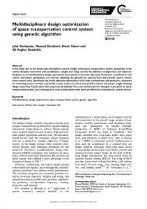
Aerodynamic shape and aerostructural design optimizations that maximize the performance at a single flight condition may result in designs with unacceptable off-design performance. While considering multiple flight conditions in the optimization improves the robustness of the designs, there is a need to develop a way of choosing the flight conditions and their relative emphases such that multipoint optimizations reflect the true objective function. In addition, there is a need to consider uncertain missions and flight conditions. To address this, a new strategy to formulate multipoint design optimization problems is developed that can maximize the aircraft performance over a large number of different missions. This new strategy is applied to the high-fidelity aerostructural optimization of a long-range twin-aisle aircraft with the objective of minimizing the fuel burn over all the missions it performs in one year. This is accomplished by determining 25 flight conditions and their respective emphases on drag and structural weight that emulate the fuel-burn minimization for over 100 000 missions. The design optimization is based on the computational fluid dynamics of a full aircraft configuration coupled to a detailed finite element model of the wing structure, enabling the simultaneous optimization of wing aerodynamic shape and structural sizing leading to optimal static aeroelastic tailoring. A coupled adjoint method in conjunction with a gradient-based optimizer enable optimization with respect to 311 design variables subject to 152 constraints. Given the high computational cost of the aerostructural analysis, kriging models are used to evaluate the multiple missions. The results show that the multipoint optimized design reduced the total fuel burn by 6.6%, while the single-point optimization reduced it by only 1.7%. This capability to analyze large numbers of flight conditions and missions and to reduce the multimission problem to a multipoint problem could be used with a few modifications to minimize the expected value of any objective function given the probability density functions of the flight conditions.
Nomenclature α
angle of attack
η
tail rotation angle
CˆL
kriging approximation for the aerodynamic coefficient, where L could also be D or My
λ �
objective-function weight for the structural weight Ws CˆD
�
W fuel C
µi
�
µi
perturbed kriging model used to compute µi perturbed weighted average fuel burn used to compute µi , where µi could also be λ
candidate flight-condition set for the selection procedure
S
sample set for kriging model training
µi
objective-function weight for a drag value Di
1
W fuel Φ xcj φjt
weighted average fuel burn �
weighted distance metric for the jth candidate flight condition weighted distance between the jth candidate flight condition and the tth selected flight condition
ρ
atmospheric density
MAC
mean aerodynamic chord
ζ
fuel fraction
CD
drag coefficient
CL
lift coefficient
Cp
pressure coefficient
cT
thrust-specific fuel consumption (TSFC)
CMy
pitching moment coefficient
D
drag force
djt
Euclidean distance between jth candidate flight condition and tth flight condition
f4DH
relative frequency of flight condition
fobj
objective function
k fPR
representative mission’s relative frequency in the payload-range diagram
Kn
static margin
L
lift force
L/D
lift-to-drag ratio
M
number of single-point objectives included in the multi-point objective function
N
number of flight conditions considered in the multi-point optimization
Ns
number of samples for kriging model training
Nintervals number of intervals for the numerical integration to solve the range equation R
mission range
Sref
reference wing area
T
thrust
V
velocity
W
aircraft weight
Wf
segment’s final weight
Wi
segment’s initial weight
Ws
structural weight
Wfuel
amount of fuel burned for a single mission
WTO
takeoff weight 2
WZF
zero-fuel weight
xcg
center of gravity location
xLE
leading edge location
xref
location of reference point to compute pitching moment
xcj
jth candidate flight condition for the selection procedure
1
Introduction
The International Civil Aviation Organization (ICAO) Programme of Action on International Aviation and Climate Change targets a 2% improvement in global fuel efficiency annually until the year 2050 [1]. At the same time, the demand for commercial aviation is expected to continue increasing at an average annual rate of 4.8% through 2036 [1]. This growth in air traffic will have an environmental impact in terms of noise, air quality, and climate change. The aviation sector currently contributes to approximately 3% of global anthropogenic carbon emissions [2], which correlate directly with fuel burn. This contribution may increase to 15% by 2050, as suggested in the 1999 Intergovernmental Panel and Climate Change (IPCC) report [3]. ICAO predicts an annual increase of 3–3.5% in global aircraft fuel consumption [1]. When designing aircraft, airframe manufacturers seek the right compromise between acquisition cost and cash operating cost (COC). The acquisition cost can be correlated with aircraft empty weight. The COC is determined by the block time and the fuel burn. The block-time contribution can be reduced by increasing the cruise speed, but this eventually increases the fuel-burn contribution to the point where the total COC increases. Thus, the best cruise speed is determined by balancing these two contributions, and the right balance depends directly on the price of fuel. Fuel burn, in turn, depends on both empty weight and drag. The consequence of this is that, when the fuel price increases (or when there is more pressure to reduce carbon emissions), the balance is steered toward better fuel efficiency and thus toward lower drag. Balancing these aircraft design tradeoffs is a complex task, since changing the parameters in one discipline affects the performance of other disciplines. Multidisciplinary design optimization (MDO) can assist the design of complex engineering systems by accounting for the coupling in the system and automatically performing the optimal interdisciplinary tradeoffs [4]. MDO has been extensively used in aircraft design applications [5, 6], especially in the design of the wing, where the coupling between aerodynamics and structures is particularly important. The earliest efforts in wing aerostructural optimization used low-fidelity models for both disciplines [7, 8]. In subsequent work, procedures that optimize the aerodynamics and the structures in sequence have been shown to fail to converge to the optimum of the MDO problem [9, 10]. Since these early contributions, the fidelity of aerodynamic and structural models has evolved immensely, which has led researchers to develop methods for high-fidelity aerostructural optimization [11, 12, 13, 14, 15, 16, 17]. Using high-fidelity MDO is a promising way to further refine conventional concepts, but MDO can be even more useful in the design exploration of unconventional aircraft configurations and new technologies. Unconventional designs such as the double-bubble and blended-wing-body concepts have recently been explored using MDO techniques to determine the potential for fuel-burn reduction [18, 19, 20, 21, 22]. Early work in wing optimization focused on drag minimization with respect to aerodynamic shape considering a single flight condition [23, 24, 25, 26]. Single-point optimization has the tendency to produce designs with optimal performance under the selected flight condition at the expense of serious performance degradation under off-design conditions [27]. Drela [28] discussed the effects of adding flight conditions on the drag minimization of airfoils in the low-speed and transonic flight regimes. He concluded that single-point drag minimization is insufficient to embody the real design requirements of the airfoil. Some researchers have explored more realistic designs that consider the performance under multiple flight conditions simultaneously for both airfoils [29] and aircraft configurations [27, 30]. Lyu and Martins [31, 32] showed a marked difference between single-point and multipoint results in the Navier–Stokes-based aerodynamic shape optimization of a transonic wing similar to the one considered herein. Buckley et al. [33] performed a multipoint optimization to obtain an optimum airfoil design; they considered 18 flight conditions. Toal and Keane [34] performed a multipoint aerodynamic design optimization with the objective of minimizing the weighted sum of drag coefficients under up to four design flight conditions. In these efforts, the multiple flight conditions are either perturbations of the nominal cruise condition (to obtain designs that are less sensitive to the flight conditions) or flight conditions based on design experience and intuition (in 3
the hope of capturing the effects of a much wider range of conditions). The weights associated with these conditions are either constant across the cases or varied based on engineering judgment. The problem with these approaches to choosing the flight conditions and respective objective weights is that there is no guarantee that they produce results that reflect real-world performance. Thus, there is a need for a new strategy to systematically choose the flight conditions and weights such that the objective function accurately represents reality. Another shortcoming of the aerodynamic shape optimization research previously cited is that it does not consider the weight tradeoffs due to the aerostructual coupling in both analysis and design. Furthermore, for multipoint design, the shape of the wing varies significantly between the various flight conditions, while aerodynamic shape optimization assumes that the shape remains fixed. Kenway and Martins [17] performed multipoint aerostructural optimization (with equal weighting for each condition) to take these coupling effects into account and obtain optimal multipoint static aeroelastic tailoring. For the aforementioned reason, we need to consider the coupling of the aerodynamic and structural disciplines to design fuel-efficient aircraft. In addition, computational fluid dynamics (CFD) is required to model the transonic aerodynamics, and a detailed structural model is required to model the effect of aerodynamic shape on the structural weight. However, such high-fidelity aerostructural analysis is costly, and it would be intractable to consider thousands of flight conditions. To address the needs previously stated, we propose a multimission, multipoint approach that automatically selects the flight conditions and their associated weights, or the relative emphases, to derive an objective function representative of the real-world performance. We use high-fidelity models in this approach. To reduce the computational cost, we use kriging surrogate models in the fuel-burn computation. This paper is structured as follows. In the next section we describe the optimization formulation and the numerical optimization algorithm. The flight mission data used in this work are detailed in Sec. 3. The methods used for the performance analysis, selection of flight conditions, and aerostructural optimization are described in Sec. 4. We then present the results and a discussion in Sec. 5, followed by a summary of what we have achieved.
2
Optimization Problem Description
In this work, we investigate the merits of performing a multimission, multipoint optimization, as compared to a single-point optimization, in the context of high-fidelity aerostructural optimizations for aircraft design. Figure 1 illustrates the high-fidelity aerostructural optimization procedure using an XDSM (eXtended Design Structure Matrix) diagram [35]. The thin black lines and thick gray lines in the XDSM diagram represent the process flow and the data dependencies, respectively. For more details on the XDSM diagram conventions, see Lambe and Martins [35]. The design variables for this optimization (xopt ) include the global variables (xglobal ), aerodynamic variables (xaero ), and structural thickness variables (xstruct ). The symbols fobj and c represent the objective function and vector of constraints in the optimization problem, respectively. At each iteration, a multidisciplinary analysis (MDA), which consists of a coupled aerodynamic and structural analysis, is performed under the selected flight conditions, where the corresponding Mach number and cruise altitude are specified. Once the aerostructural analysis has converged, the aerodynamic discipline computes the aerodynamic drag, and the structures discipline computes the wing structural weight. These values are then used in the objective-function evaluation, with constant weights µi and λ. This procedure is repeated until the optimizer finds an optimum. Each component of this optimization procedure is described in detail in this section. 2.1 Objective Function In this optimization problem, we seek to minimize the weighted average fuel burn over a large set of flight missions for a long-range twin-aisle aircraft configuration. The objective-function formulations for both the single-point and multipoint optimization are described below. 2.1.1 Multipoint Optimization In a multipoint optimization, the objective function, fobj , is expressed as the weighted combination of the quantity of interest fj evaluated under each condition j, M X fobj = wj fj , (1) j=1
4
x∗opt
xopt
(Mach, Altitude)i
Optimization
xglobal xaero MDA
ˆ struct y
∗ yaero
yaero
Aerodynamic analysis
∗ ystruct
ystruct
µi , λ xglobal xstruct
yaero
Di
Structural analysis
Ws PN
fobj , c
i=1
µi Di + λWs
Figure 1: XDSM diagram for the coupled aerostructural optimization procedure. where wj are the user-specified weights, and M denotes the number of conditions considered in the objective-function evaluation. The designer must choose appropriate weights so that the objective function accurately reflects the intended operation. As mentioned in the Introduction (Sec. 1), the choice of these weights is one of the difficulties in multipoint optimization, and usually they are chosen rather arbitrarily without any quantitative rigor. We address this difficulty by developing a quantitative method for systematically determining the weights. To determine the fj and wj in the context of our optimization problem, we first express our objective function (fuel burn) as a function of drag values (Di ) under different flight conditions (i = 1, 2, . . . , N ) and the structural weight (Ws ), fobj = f (D1 , D2 , . . . , DN , Ws ) .
(2)
We can then linearize this objective function to obtain fobj ≈
N X ∂fobj i=1
∂Di
Di +
∂fobj Ws . ∂Ws
(3)
Using µi and λ to represent the derivatives of the objective function with respect to Di and Ws , respectively, we can write N X µi Di + λWs . (4) fobj ≈ i=1
Using the general multipoint formulation conventions (1), we have M = N + 1, where the Di ’s and Ws are the fj ’s, and correspondingly the µi ’s and λ are the wj ’s. In the current work, N is set to 25. As previously mentioned, the objective function in this work is the weighted average fuel burn from hundreds of representative missions, selected from over 100 000 actual flight missions. For each representative mission, a detailed mission analysis is performed to compute fuel burn. This analysis procedure is described in Sec. 4.1, and the flight conditions for which the Di ’s are computed are selected based on the procedure presented in Sec. 4.3. 2.1.2 Single-point Optimization For the single-point optimization problem, only one flight condition is considered. The amount of fuel burned is computed using the classical Breguet range equation [36, 37], � � W1 V L ln , (5) R= cT D W2 5
where R is the mission range, V is the cruise speed, and cT is the thrust-specific fuel consumption (TSFC). The lift-todrag ratio is L/D, and the initial and final weights are represented by W1 and W2 , respectively. Since we consider the fuel burn during only a single cruise segment, we assume W1 to be equal to the maximum takeoff weight (MTOW). The final cruise weight, W2 , is obtained by adding the operating empty weight and the payload. The initial weight can be found by rearranging the range equation (5), � � cT D . (6) W1 = W2 exp R V L The fuel burn can then be computed by taking the difference between the initial and final weights, Wfuel = W1 − W2 ,
(7)
which is our objective function, fobj . A linearized objective function is then derived for the single-point optimization case, in a similar fashion to the multipoint optimization case, fobj ≈
∂fobj ∂fobj D+ Ws ≈ µD + λWs . ∂D ∂Ws
(8)
The objective function for the single-point optimization is expressed in the general multipoint optimization formulation (1), with M = 2 to allow for a suitable comparison with the multipoint optimization. 2.2 Baseline Aircraft The initial geometry for the optimization is given by the common research model (CRM) [38] wing-body-tail configuration, shown in Fig. 2. This figure shows an aerostructural solution at Mach = 0.84. Outer mold line shows the 1g cruise shape with the pressure coefficient distribution (right), and finite element model shows the 2.5g deflections and failure criterion on the upper skin, lower skin, ribs, and spars (left). The stress values are normalized with respect to the yield stress. This aircraft exhibits design features typical of a transonic wide-body long-range aircraft. It was designed to exhibit good aerodynamic performance across a range of Mach numbers and lift coefficients. Since the CRM geometry defines only the outer mold line shape, we use a structural model similar to that created by Kenway et al. [16] and shown in Fig. 3. The wing structure conforms to the wing outer mold line and is representative of a modern airliner wingbox. In addition to the aerodynamic and wing structural models, we require MTOW and other parameters
Figure 2: Aerostructural solution, showing the structural stresses (left) and the pressure coefficient distribution (right). to perform the mission analysis. The overall dimensions of the CRM are similar to those of the Boeing 777-200ER, so
6
we use publicly available data for this aircraft to complete the missing information1 . Table 1 lists the key additional parameters used for the optimizations. Table 1: Aircraft specifications Parameter
Value
Nominal cruise Mach number Nominal cruise lift coefficient Span Aspect ratio Mean aerodynamic chord (MAC) Reference wing area Sweep (leading edge) Maximum takeoff weight (MTOW) Operational empty weight Design range Initial wing weight Secondary wing weight Fixed weight Thrust-specific fuel consumption (cT )
0.84 0.5 58.6 9.0 7.3 383.7 37.4 298 000 138 100 7 725 29 200 8 000 100 900 0.53
Units – – m – m m2 deg kg kg n mile kg kg kg lb/(lbf · h)
2.3 Design Variables In the multipoint optimization, we consider 311 design variables. Table 2 lists all the optimization variables, split between global variables and local disciplinary variables (aerodynamics and structures). The number of aerodynamic design variables for the single-point optimization is lower, since only one cruise condition is considered. Thus, we have three angles of attack and tail rotations each, one for cruise and two for the maneuver conditions. The global and structural thickness variables for the single-point optimization are the same as those for the multipoint optimization. Table 2: Design variables for the multipoint optimization case. Global variables Description Span Sweep Chord Twist Shape Total
Aerodynamic variables
Quantity 1 1 3 5 96 106
Description
Quantity
Structural thickness variables Description
Quantity
Angle of attack Tail rotation
27 27
Upper skin and stringers Lower skin and stringers Ribs Spars
36 36 6 73
Total
54
Total
151
Grand total
311
A free-form deformation (FFD) volume approach is used for the geometric parameterization; further details are provided by Kenway and Martins [17]. The main wing planform variables of span, sweep, chord, and twist are all global variables, since they directly affect the geometry in each discipline. The geometric design variables and the mesh discretization used for the optimization are shown in Fig. 4. Chord design variables manipulate FFD coefficients at the root, Yehudi break, and tip sections. The remaining sections are linearly interpolated. Five twist angles are defined similarly. For the chord and twist variables, the actual geometric perturbation is cubic because of the order of FFD in the span-wise and chord-wise directions. A single sweep variable sweeps the leading edge of the wing. The shape variables are used to perturb the coefficients of the FFD volume surrounding the wing in the z (normal) direction, thus prescribing the airfoil shapes. 1
Boeing Commercial Airplanes, 777-200/200ER/300 airplane characteristics for airport planning (Document D6-58329), http://www.boeing.com/boeing/commercial/airports/777.page. (Accessed 23 August 2013.)
7
Figure 3: Structural thickness design variable groups; each colored patch represents a structural thickness variable.
Figure 4: Geometric design variables and FFD volumes (left) and CFD surface mesh (right). The structural design variables are shown in Fig. 3, where each colored patch represents a structural thickness variable. The thicknesses of the skin and stringers are set to be equal within a given patch. This results in 36 design variables for the upper skin and stringers and 36 for the lower skin. There are 6 design variables for the ribs and 73 for the spars. Since no sized structure is provided for the CRM model, we must determine a reasonably efficient initial structural model to enable comparisons between the initial and optimized designs. The design of the initial structure is generated by performing a stress-constrained mass-minimization optimization using fixed aerodynamic loads.
8
2.4 Design Constraints In this section we describe the constraints that are used for the aerostructural optimization. We divide the constraints into three groups: geometric constraints, aerodynamic constraints, and structural constraints, as listed in Table 3. Table 3: Design optimization constraints Geometric/target constraints Description
Aerodynamic constraints
Quantity
Description
tLE /tLEInit ≥ 1.0 tTE /tTEInit ≥ 1.0 A/Ainit ≥ 1.0 VWing Box /VWing Boxinit ≥ 1.0 tTE Spar ≥ 0.20 tTip /tTipInit ≥ 0.5 M AC = M AC ∗ xcg = x∗cg tWing Box /tWing Boxinit ≤ 1.1
11 11 1 1 5 5 1 1 55
Cruise: Cruise: Maneuver: Maneuver: Static margin:
Total
91
Total
Structural constraints Quantity
∗
L=L ∗ CM y = CM y L=W CMy = 0.0 Kn ≥ 0.25
Description
25 25 2 2 1
2.5 g Lower skin: 2.5 g Upper skin: 2.5 g Ribs/spars: 1.3 g Lower skin: 1.3 g Upper skin: 1.3 g Ribs/spars:
55
Total
KS KS KS KS KS KS
Quantity ≤ 1.0 ≤ 1.0 ≤ 1.0 ≤ 0.42 ≤ 1.0 ≤ 1.0
Grand total
The first two geometric constraints tLE and tTE are used to limit the initial wing thickness at the 2.5% and 97.5% chord locations, which effectively constrain the leading-edge radius and prevent crossover near the sharp trailing edge. The purpose of constraining the leading-edge radius is twofold: first, it eliminates excessively sharp leading edges, which are difficult to manufacture, and second, it ensures that the aerostructural optimization does not significantly impact the low-speed CLmax performance, which is largely governed by the leading-edge radius. We constrain the projected wing area A to be no less than the initial value to prevent a degradation of landing and takeoff field performance. We also constrain the internal wing box volume VWingBox to be no less than the initial value to ensure sufficient wing fuel-tank capacity. Several additional thickness constraints are also enforced. Minimum trailing-edge spar height constraints tTE spar are enforced over the outboard section of the wing. This constraint ensures that adequate vertical space is available for the flap and aileron attachments and actuators. Maximum thickness constraints tWingBox are enforced to prevent excessively thick transonic sections with strong shocks, causing severe flow separation. Since shock-induced flow separation is not modeled with the Euler equations, we use these constraints to help enforce this physical constraint. The final thickness constraint ttip is used to ensure that the optimization does not produce an unrealistically thin wingtip. The solution for each cruise condition is trimmed based on the weight of the aircraft under each condition. The two maneuver conditions used as load cases for the structural sizing are a 2.5g symmetric pull-up maneuver (the limit load for the wing structure) and a 1.3g acceleration to emulate gust loads, with a stress constraint based on a fatigue limit. The static margin (Kn ) at a cruise condition is constrained to be greater than 25% with the reference center of gravity (c.g.) location at 10% of the mean aerodynamic chord (MAC). We use the following approximation to estimate the Kn of a deformed configuration [39]: CMα Kn = − , (9) CLα where CMα and CLα are the derivatives of the moment and lift coefficients with respect to the angle of attack, respectively. Lastly, we must constrain the structural stresses. We use the Kreisselmeier–Steinhauser (KS) constraint aggregation technique [40, 41], which can be written as "K # X 1 ln exp [ρKS (fk (x) − fmax )] . (10) KS (x) = fmax + ρKS k=1
In this work, the functions fk (x) and fmax refer to the stress values and yield stress, respectively. The aggregation parameter ρKS is set to 80. This KS function combines the thousands of stress constraints into just three functions. 9
1 1 1 1 1 1
6 152
The first KS constraint corresponds to the lower wing skin and stringers, the second is for the upper wing skin and stringers, and the third is for the spars and ribs. For the upper wing skin, which is dominated by compression, we use Aluminum 7050, which has a maximum allowable stress of 300 MPa. The remainder of the primary wing structure uses Aluminum 2024, which has a maximum allowable stress of 324 MPa. For the 2.5g maneuver condition, the maximum von Mises stress must be below the yield stress, which requires the three KS functions to be less than 1.0. The 1.3g maneuver constraint is used to emulate a fatigue criterion due to gusts for the lower wing skin and stringers, which are under tension during normal loading. We limit the stress on the lower wing skin and stringers to be less than or equal to 138 MPa for this load condition. The value is selected considering the fatigue stress limit for Aluminum 2024. The upper limit for this KS function is 0.42. The remaining two KS functions for the 1.3-g maneuver condition retain the maximum KS value of 1.0. 2.5 Optimization Algorithm Because of the costly nature of multipoint optimization, it is desirable to use a gradient-based optimization method to reduce the number of function evaluations necessary to reach a local optimum. The coupled adjoint method allows us to compute the gradients of the functions of interest with respect to hundreds of design variables very efficiently. Kenway et al. [16] gave the details of the accuracy, computational cost, and parallel performance of this approach, while Martins and Hwang [42] provided an overview of the methods available for computing coupled gradients. The optimizer we use is SNOPT, an optimizer based on the sequential quadratic programming approach [43], through the Python interface provided by pyOpt [44]. 2.6 Computational Resources The aerostructural optimization is performed on a massively parallel supercomputer equiped with Intel Xeon E5540 processors connected with a 4x-DDR nonblocking InfiniBand fabric interconnect [45]. Each aerostructural solution is computed in parallel, and all flight solutions are computed in an embarassingly parallel fashion [46] (i.e., each flight condition is computed in a different set of processors). Each of the cruise and stability flight conditions uses 32 aerodynamic processors and 4 structural processors, while each maneuver flight condition uses 40 aerodynamic processors and 16 structural processors. A variable number of processors for the different conditions is required for good load balancing, since the maneuver conditions must solve for five adjoint vectors (lift, moment, and the three KS functions), while the cruise conditions compute only three adjoint solutions (lift, drag, and moment). The total number of processors used to perform the multipoint optimization is thus 36 × 25 + 36 + 56 × 2 + 1 = 1049. The last term represents a single additional processor that computes the viscous drag as described in Sect. 4.2. To help reduce the computational cost, we use different computational meshes for the different flight conditions. The cruise and stability conditions use a 1.8-million-cell CFD mesh and a 209 430 degree-of-freedom (DOF) structural mesh comprising 37 594 second-order mixed interpolation of tensorial components (MITC) shell elements. The maneuver condition uses a 1.0-million-cell CFD mesh and a third-order version of the same structural mesh consisting of 869 754 DOF with the same number of elements. Using different mesh sizes reduces the overall computational cost by allowing coarser meshes in analyses for which the reduction in spatial accuracy does not adversely affect the result. For the cruise conditions, only accurate displacements are required, since no KS functions are evaluated for these conditions. Conversely, for the maneuver conditions, accurate predictions of drag are not required, and the coarser CFD grids are sufficiently resolved to generate load distributions that are accurate enough.
3
Flight Mission Data
To obtain a set of missions that is representative of the actual operations of a given aircraft model, we consulted the BTS flight database2 . We extracted payload and range data for all Boeing 777-200ER flights that took off from the United States, landed in the United States, or both. These data consist of a set of 101 159 flights for which the payloadrange frequency histogram is shown in Fig. 5. This histogram was plotted using a 25 × 50 grid of bins. Each bin is 291 n mile in range by 1 t in payload. For each bin that contains at least one flight mission, we chose the midpoint to represent the range and payload of that bin. This resulted in 529 representative flight missions for our analysis. The black circle in Fig. 5 represents the flight condition used in the single-point optimization (a 5 000 n mile range and 30 000 kg payload mission). The color map shown in this histogram represents the number of flight missions contained within each bin (the frequency). By normalizing this frequency information with respect to the total number of flight 2
TranStats, Bureau of Transportation Statistics http://www.transtats.bts.gov/. (Accessed 23 August 2013.)
10
k missions, we can derive the relative frequency for each bin, fPR , which is to be used when computing the weighted average fuel burn (we explain this in more detail in Sec. 4.1).
Frequency 1504 1377 1249 1121 994 866 738 611 483 355 228 100
Payload (1000 kg)
50
40
30
20
10
0
0
2000
4000
6000
8000
Range (nmi)
Figure 5: Histogram of 101 059 flights for the Boeing 777-200ER aircraft and its payload-range envelope. The black circle represents the mission used for the single-point optimization. The cruise Mach number and the c.g. locations are not available in the mission database, so we estimate values for these parameters using probability density functions (PDFs). The PDFs for these two parameters are selected to reflect the actual aircraft operation. Since information on the actual Mach number during flight is not available, the mission Mach number is assumed to have a normal distribution with the mean equal to the nominal cruise Mach number, 0.84, and a standard deviation of 0.0067. The normal variation around the nominal value accounts for the unknown operational demands that might require faster or slower flight. The assumed standard deviation is deemed realistic to model this variation in our optimization problem. The c.g. location xcg is expressed as a percentage of MAC, measured from the leading-edge location xLE . We assume that the c.g. location PDF is a uniform distribution centered at 27.5% MAC, with an interval defined by subtracting and adding 10% MAC to this value. Thus, we can write these two PDFs as Mach ∼ N (0.84, 0.0067) ,
xcg ∼ xLE + U (0.175, 0.375) · MAC,
(11)
where N and U are the normal and uniform distributions, respectively. A further uncertain parameter is introduced in the cruise altitude. A ±1000 ft variation is added to the computed altitudes to simulate the variability in the altitudes assigned by air traffic control.
4
Solution Methods
This section describes the methods used to solve the optimization problem described in Sec. 2. We first present the mission-analysis procedure to compute the amount of fuel burned, followed by the aerodynamic coefficient approximation with kriging models. We then discuss the detailed procedure to select the flight conditions, and finally we describe the aerostructural optimization framework. 4.1 Fuel-Burn Computation The fuel burn for each flight mission is computed by performing mission analysis. For this analysis, the flight mission is divided into five segments: takeoff, climb, cruise, descent, and landing, as illustrated in Fig. 6. The takeoff and zerofuel weights are denoted WTO and WZF , respectively. The zero-fuel weight comprises the operating empty weight and payload (passengers, luggage, and cargo). The cruise segment is assumed to include step climbs when the cruise range is longer than 1 000 n mile. We first determine the number of cruise subsegments by assigning a subsegment for each 1 000 n mile of cruise range to simulate the step-climb procedure during cruise. The altitude at each step is computed
11
W3 W2
Cruise
Descent
Climb
WTO
Takeoff
W1
W4
Landing
WZF
Figure 6: Flight mission profile. such that it corresponds to a target lift coefficient, which is achieved via the secant method. The maximum altitude is set to 41 000 ft. The relation between the flight altitude and CL is given by L=
1 ρSref V 2 CL , 2
(12)
where Sref is the reference wing area. The atmospheric density ρ and the speed of sound, which determine the flight speed (V ) at a given Mach number, are computed using the standard atmospheric model (US Atmosphere 1976) as functions of cruise altitude. Since we assume steady level flight, we set the lift force to be equal to the initial weight at each subsegment. Since we do not use an engine model, we do not account for thrust lapse and assume that sufficient excess thrust is available to achieve the flight conditions of all the missions. To compute the fuel burned during a mission, we use assumed fuel fractions for the takeoff, climb, descent, and landing segments. The fuel fraction, ζ, refers to the amount of fuel burned in the segment as a fraction of the segment’s initial weight. The general equation to find the segment’s final weight given its initial weight and fuel fraction is Wf = (1 − ζ) Wi ,
(13)
where Wi and Wf refer to the segment’s initial and final weights, respectively. This equation is used to compute W1 given WTO and ζtakeoff , W2 given W1 and ζclimb , W4 given W3 and ζdescent , and WZF given W4 and ζlanding . The assumed fuel fractions are listed in Table 4. Table 4: Fuel fraction values Segment Fuel fraction, ζ
Takeoff
Climb
Descent
Landing
0.002
0.015
0.003
0.003
For the cruise segment, a numerical integration of the range equation is performed to compute the cruise fuel burn, which corresponds to W2 − W3 . As previously mentioned, we do not use an engine model and thus assume constant TSFC (cT ) for all cruise flight conditions, cT =
Weight of fuel burned per unit time (N/s) . Unit thrust (N)
(14)
The rate of reduction of the aircraft weight can thus be computed as dW = −cT T, dt
(15)
where W is the aircraft weight, and T is the thrust. Now we can express the range R as a definite integral of aircraft speed V over a time interval, Z t2 R= V dt. (16) t1
Substituting Eq. (15) into Eq. (16), we can define the flight range given the specific range (the range per unit weight of fuel, −V /cT T ) using the following equation: Z W3 V R= − dW . (17) cT T W2 12
Approximating the preceding range equation by numerical integration, we obtain R≈
NX intervals n=1
� V (n) � (n) (n) W − W , i f cT T (n)
(18)
where the superscript (n) refers to the indices of the intervals (n = 1, . . . , Nintervals ) used to integrate the cruise segment (n) (n) of a particular mission. The initial and final weights of interval n are denoted by Wi and Wf , respectively. Each evaluation of the range equation assumes a value of takeoff gross weight, which comprises the zero-fuel weight and the fuel weight. At each evaluation, we compute the range achieved using the available fuel. We then iterate this evaluation using the secant method to match the actual range to the target mission range, thus finding the fuel burn for a specified mission range. We can then obtain the amount of fuel burned during the cruise segment as Wfuel = W2 − W3 .
(19)
Now we use the numerical integration (18) to evaluate the cruise range. Each cruise subsegment (i.e., each step in the step-climb procedure) is further divided into 10 intervals, as illustrated in Fig. 6, where each cruise interval burns an equal amount of fuel. We set Nintervals in the numerical integration to be equal to the number of subsegments times the number of intervals per subsegment. The initial and final weights for each interval can be found given W2 , W3 , and Nintervals . We need only T (n) to complete the evaluation. Assuming steady level flight, D(n) = T (n) and (n) L(n) = Wi . We can compute D(n) by performing aerostructural solutions for which the angle of attack is varied to match the target lift. To ensure that the aircraft is trimmed, we also enforce CMy = 0. We use a Newton method to find the angle of attack (α) and tail rotation angle (η) that satisfy these two conditions simultaneously. The computation of the mission fuel burn using the above procedure would require a large number of high-fidelity aerostructural solutions. We can get an estimate of the number of solutions required by multiplying the number of missions, the number of intervals, the number of secant iterations, and the number of Newton iterations. Since we consider hundreds of representative missions with dozens of intervals for each mission, this analysis would easily require millions of aerostructural solutions. Therefore, kriging models are built to approximate the aerodynamic force and moment coefficients (CL , CD , and CMy ) that are used in the mission analysis computation. By constructing kriging models for these coefficients, we significantly reduce the required number of high-fidelity function calls to just the number of samples required to build the surrogates (25 in this case), thus making the procedure computationally tractable. The surrogate model to approximate CMy is constructed using high-fidelity aerostructural analyses on kriging sample points. These analyses assume a fixed c.g. location. Therefore, we add a deviation of pitching moment to accommodate the varying c.g. locations of the different missions, ∆My = W (xcg − xref ) ,
(20)
where xref is the location of the reference point used to compute the pitching moment. This deviation leads to a correction in the pitching moment coefficient, ∆CMy =
∆My . · MAC
1 2 2 ρSref V
(21)
The procedure presented here computes the fuel burn corresponding to one flight mission. To find the weighted k average fuel burn, W fuel , from the 529 representative missions, we use the relative frequency fPR , yielding W fuel =
Nrep X
k k fPR Wfuel .
(22)
k=1
In our optimization formulation, all mission analyses are performed and completed prior to the optimization procedure. Using these analysis results, we determine the flight conditions to be included in the objective function (4) and derive the corresponding objective-function weights. The procedure is described in more detail in Sec. 4.3.
13
4.2 Aerodynamic Coefficient Approximation For the mission analysis, three kriging models are created for CL , CD , and CMy with respect to the following inputs: Mach number, altitude, angle of attack, and tail rotation angle. The kriging approximation method is a statistical interpolation method based on Gaussian processes. Kriging surrogate models belong to the data-fit black-box surrogate modeling classification [47], which relies on samples from the functions to be approximated in the model construction [48, 49, 50]. The ranges for these kriging inputs are listed in Table 5. These inputs are normalized to be between 0 and 1 for the kriging construction and approximation, since they have significantly different scales (e.g., between altitude and Mach number). The drag coefficients approximated by kriging models are only inviscid drag coefficients. To obtain the total drag coefficient, we add a constant viscous drag coefficient of 0.0136. The same value is used in the total drag computation corresponding to all flight conditions of all missions. This viscous drag is computed based on a flat-plate turbulent skin friction estimate with form factor corrections. The van Driest II method [51] is used to estimate the skin friction coefficient; Kenway and Martins [17] described this estimate in more detail. Note that this value is used only in the mission analysis procedure with the initial design, which is performed prior to the optimization. During the optimization, this value is updated as the wing area changes. Input variable
Lower bound
Upper bound
Mach Angle of attack Altitude Tail angle
0.80 0◦ 29 000 ft −2◦
0.86 3◦ 41 000 ft 2◦
Table 5: Ranges for the surrogate model input variable values. There is no general rule to assess the number of samples required to achieve a desired accuracy in a kriging model, which is problem dependent. In our case, we determine that 25 samples are a good compromise between computational cost and the accuracy of the kriging surrogate models; this will be further discussed when we present the results. To quantify the accuracy of the kriging surrogate model, we use the leave-one-out cross-validation strategy. The cross-validation root-mean-squared error (CVRMSE) is computed using the formula of Mitchell and Morris [52]. Following this procedure, one sample is removed at a time, and it is predicted by the kriging model constructed using the remaining (Ns − 1) samples, where Ns denotes the number of samples. The discrepancy between the predicted value and the actual value at sample xi is denoted ei . The CVRMSE can then be computed as follows: v u Ns u 1 X CVRMSE = t e2 . (23) Ns i=1 i To evaluate the accuracy, we compute the normalized CVRMSE values for the kriging models, where the computed CVRMSE is normalized with respect to the range (the difference between the maximum and minimum values) of the approximated variable. This normalization provides a better idea of the relative magnitude of this error with respect to the quantity of interest. The kriging model validations will be discussed in Sec. 5.2.
4.3 Flight Condition Selection Procedure Our main goal is to develop a weighted objective function based on a limited number of flight conditions that emulates the fuel burn of all the flight missions being considered. In this section, we explain the procedure that selects the flight conditions, as well as the corresponding weighting factors. We start with an overview, and we then present the details of the algorithm. The main goal of this procedure is to select the N flight conditions used in the objective-function evaluation (where the drag values, Di , i = 1, . . . , N , are evaluated) and the corresponding weights required to form the objective function (4). As mentioned in Sec. 2.1, the objective-function weights, µi and λ, are the gradients of the weighted average fuel burn W fuel (22) with respect to the drag values, Di , and structural weight Ws , respectively. Our fuel-burn computation uses kriging models in the mission analysis, and thus we can express W fuel as a function of the samples used to construct the kriging models. We can then use the kriging samples (in the four-dimensional space of Mach number, angle of attack, altitude, and tail rotation angle) as the flight conditions in the linearized objective function (4). 14
The linear objective weights, µi and λ, are computed using the finite-difference method. For this computation, each � CD sample value is perturbed, and the corresponding perturbed weighted average fuel burn, W fuel µi , can then be computed. The weight µi can then be computed using the following relation: µi =
∂fobj ∂W fuel ∂W fuel 2 . = = ∂Di ∂Di ρSref V 2 ∂CDi
(24)
The objective-function weight for Ws , λ, is obtained in a similar manner except that Ws is perturbed instead. To construct the kriging model, we require a strategy for selecting the sample points. We start by using Halton sampling [53], which is a space-filling low-discrepancy method. The discrepancy in this case is the departure of the sampling points from a uniform distribution, thus ensuring an even distribution of samples over the design space [53]. Instead of relying on Halton sampling throughout, we want a sampling procedure that is biased toward regions in the space of flight conditions where more evaluations are required in the course of the aircraft mission analyses. To achieve this, we require the flight-condition distribution. Based on this rationale, we perform two sets of mission analyses. The first set is performed to obtain the flight-condition distribution, which is also the distribution of points in the kriging input space that are evaluated to complete the mission analyses. Based on this information, the final samples are selected. The second set is performed to compute the linearized objective-function weights, µi and λ. This procedure is described in further detail next. Fig. 7 shows the XDSM diagram that illustrates this procedure. The step-by-step procedure is listed next with a numbering consistent with that shown in the diagram. 1. Evaluate CL , CD , CMy at the 25 Halton sample points by running the high-fidelity analyses. 2. Build kriging models of the aerodynamic coefficients (CˆL , CˆD , CˆMy ) using these samples. 3. Perform mission analyses for the 529 representative missions using the kriging models and store all the flight conditions evaluated in these analyses to generate the four-dimensional histogram f4DH in the space of the flight conditions (Mach, α, altitude, η). 4. Perform the flight-condition selection (Algorithm 1) to select the 25 flight conditions to be used as a0 kriging samples in the second mission analysis (step 6), with which the objective function weights, µi and λ, are computed using Eq. (24); and b) flight conditions in the multipoint aerostructural optimization problem (see Sec. 5.1). 5. Build the kriging models (CˆL , CˆD , CˆMy ) using the newly selected samples (“final N samples” in Fig. 7). 6. Perform the mission analyses for all representative flight missions to compute the weighted average fuel burn, W fuel . 7. Loop through all samples, i = 1, . . . , N , to compute the gradient µi = ∂W fuel /∂Di via finite differences. i i 8. Perturb the ith CD sample value, CD ← CD + ∆CD .
� � 9. Rebuild the kriging model CˆD using the perturbed sample. This “perturbed” kriging model is written CˆD , µi
since the model is used to compute µi .
10. Perform the mission analysis to compute the perturbed weighted average fuel burn, W fuel 11. Compute µi using finite differences, µi =
W fuel
�
µi
− W fuel
∆CD
�
.
12. Perturb the structural weight, Ws ← Ws + ∆Ws . 13. Perform the mission analysis to compute the perturbed weighted average fuel burn, W fuel turbed kriging models (CˆL , CˆD , CˆMy ).
15
µi
.
(25)
�
λ
, using the unper-
Figure 7: The procedure to select flight conditions and compute weights for the multipoint objective function. 16
λ
µi
1: Sampling (Halton) CˆL , CˆD CˆM
2: KM
4: Sample Selection
Hist. of [M, α, h, η]
5: KM
Final N samples
6: MA
y
CˆL , CˆD CˆM
7:12 → 8 i=1→N 8: ∆CD
9: KM
i CD + ∆CD
CˆD
�
µi
10: MA
�
CˆL , CˆMy
�
µi
11: FD
W fuel
W fuel
KM: build kriging model, MA: mission analysis, ∆: perturb, FD: finite difference
3: MA
y
Payload, R, Ws , M , xcg , h
Initial samples
12: ∆Ws
Ws
13: MA
Ws + ∆Ws
y
CˆL , CˆD CˆM
Payload, R, M , xcg , h
�
λ
14: FD
W fuel
14. Compute λ using finite differences,
� W fuel λ − W fuel λ= . ∆Ws
(26)
When this procedure is completed, we have the flight conditions, (Mach, Altitude)i , i = 1, 2, . . . , N , and the objective-function weights (µi , i = 1, 2, . . . , N and λ) that are required in the high-fidelity aerostructural optimization shown in Fig. 1 and described in Sec. 2. We now explain the flight-condition selection procedure mentioned in step 4 above. The main idea of this procedure is to select 25 flight conditions that are 1) located in the flight-condition space area where most points are requested by the mission analysis; and 2) evenly spread out in the flight-condition space, to avoid clustering of samples in the kriging construction. This second condition is desirable because small distances between samples can lead to an ill-conditioned correlation matrix. To deduce the dominant region in the flight-condition space, we look at the four-dimensional histogram generated in step 3 above. This discrete histogram contains information on the relative frequency of the flight conditions f4DH , obtained by taking the number of evaluated flight conditions that belong to each bin in the four-dimensional space, normalized by the total number. Based on the aforementioned reasoning, we derive the sampling criteria using f4DH and the Euclidean distance between points d. The flight-condition selection procedure is summarized in Algorithm 1. This procedure adds flight conditions to the set S, which is initially empty. For this procedure, the desired number of flight conditions (also kriging samples) Ns is set to 25. Until the final flight-condition set is finalized, no high-fidelity function evaluations are required in this procedure. Algorithm 1 Flight-condition selection procedure Inputs: Ns , f4DH Output: S = {xsi }i=1,2,...,25 � 1: C = xcj j=1,2,...,500 � 2: Compute f4DH xcj ∀j � 3: Sort C based on f4DH xcj in descending order 4: xs1 = xc1 5: for i = 2 → Ns do 6: for each xcj ∈ / S do 7: for each xst ∈ S do 8: djt = kxcj − xst k2 � � 9: φjt = djt f4DH xcj + f4DH (xst ) 10: end for� P 11: Φ xcj = t φjt 12: end for 13: xsi = xcj , where j = arg max Φ (xck ) 14: xsi → S 15: end for
. Number of flight conditions and flight-condition histogram . Final set of flight conditions . Draw 500 Halton samples for the candidate points . Flight-condition frequency for each candidate point . Assign the most frequent flight condition as the first . Repeat until we obtain Ns flight conditions . Consider only flight conditions that are not in set . Loop over all previously selected flight conditions . Evaluate weighted distance . Compute weighted distance metric . Select best flight condition based on metric . Add selected point to flight condition set
� A set of candidate points, C = xcj j=1,2,...,500 , are required for this flight-condition selection procedure. For this purpose, we use 500 Halton points to fill the input space of interest � evenly with candidate points. For each candidate flight condition, the corresponding relative frequency f4DH xcj is computed by assigning the relative frequency of the bin where xcj is located. The candidate flight conditions are then sorted in descending order based on this quantity. The sample set is initialized by assigning the first candidate point as the first sample point, xs1 = xc1 (line 4 in Algorithm 1). The remaining 24 samples are added one by one using the following procedure (loop starting in line 5). At each sample addition, the algorithm selects the candidate point with the highest weighted distance metric, Φ. To compute this metric, we first need to compute the Euclidean distance between each candidate flight condition and each selected flight condition (line 8). The weighted distance for each pair of candidate and selected flight conditions is then computed, so that we can evaluate the selection metric (line 11). The algorithm is terminated when Ns samples are found. The results of this sample selection procedure for our aircraft design problem are presented in Sec. 5.1.
17
4.4 Aerostructural Optimization Most large commercial aircraft operate in the transonic flight regime during cruise. Therefore, at a minimum, we must solve the Euler equations to accurately predict the induced and wave drag. In addition, the wing is flexible, and its shape is dependent on the flight conditions. Therefore, we require static aeroelastic (aerostructural) solutions to evaluate the aircraft performance. We employ the aerostructural analysis and design optimization framework developed by Kenway et al. [16], who applied it to the aerostructural optimization of the same aircraft considered herein. However, only five flight conditions were considered in that work. The CFD solver used in this work is SUmb [54], a structured multiblock flow solver that includes a discrete adjoint solver that was developed using algorithmic differentiation [55, 56]. SUmb uses a second-order finite-volume discretization to solve the Euler equations using a preconditioned matrix-free Newton–Krylov approach. The structural solver is the Toolbox for the Analysis of Composite Structures (TACS). TACS is a parallel finite-element solver developed for the analysis and optimization of composite structures [57]. The transfer of loads and displacements is done through a consistent and conservative approach, which is based on the work by Brown [58]. A coupled adjoint method that allows us to compute the gradients of the multidisciplinary functions of interest is one of the critical components that make high-fidelity aerostructural optimization tractable for large numbers of design variables [16, 17].
5
Results
In this section, we present the results of a multimission, multipoint, high-fidelity aerostructural optimization for a longrange aircraft configuration, and we show that this formulation yields a better aggregate fuel burn than a single-point optimization. We begin by presenting the flight-condition selection results, followed by the kriging model validation for the aerodynamic coefficients (CL , CD , CMy ). We end with a comparison between the proposed approach and a single-point aerostructural optimization. 5.1 Flight Conditions The 25 flight conditions for the multipoint optimization are selected following the procedure presented in Sec. 4.3. This selection is based on the distribution of flight conditions evaluated when performing mission analyses for all 529 representative missions, which amount to a total of 21 430 flight conditions. This number is obtained by adding the numbers of the numerical integration intervals of all the representative flight missions. Recall that the number of intervals depends on the flight range of each mission, and it varies from 10 to 70. The frequency distributions of Mach number, altitude, angle of attack, and tail rotation angle from these 21 430 flight conditions are shown in the diagonal frames in the scatterplot matrix of Fig. 8. The maximum cruise altitude is set to 41 000 ft for the mission-analysis procedure, which accounts for the abrupt upper bound in the altitude histogram. The upper triangular frames of Fig. 8 show where the sample-selection procedure redistributes the 25 flightcondition samples to be concentrated around regions in the kriging input space that are more frequently evaluated when computing the weighted average fuel burn. In this scatter-plot matrix, the four-dimensional space is deconstructed into its various two-dimensional projections. The initial samples (the green triangles) cover the kriging input space almost uniformly, whereas the selected samples (the blue squares) gravitate toward the kriging input space region with high frequency values (gray circles whose sizes are proportional to the respective frequencies). The corresponding objective-function weights µi are illustrated in the lower triangular frames of Fig. 8. The black dots represent the samples with positive µi values, whereas the red dots are those with negative µi values; each dot is sized by the magnitude of µi . These 25 samples are also used to determine the cruise conditions in the high-fidelity optimization problem, which are listed in Table 6. The lift (in % MTOW) and CMy listed in this table correspond to the angle of attack α and tail rotation angle η specified at each sample point. The negative µi values imply an inverse relation between drag and fuel burn, i.e., increasing drag under these flight conditions would reduce the weighted average fuel burn, which appears counterintuitive. We investigate this issue by perturbing each of the sample points (with a positive value) and observing the effect on the drag value change in each flight condition evaluated in the mission analysis for all representative flight missions. Each perturbation alters the shape of the kriging response surface for CD . The areas close to perturbed samples have a higher CD compared to the unperturbed case, but the Gaussian process component of the kriging model may decrease the CD values in other areas further away from the perturbed sample. The net change in the weighted average fuel burn depends on where in the input space the CD changes occur. Figure 8 shows that the flight conditions with positive weights are located mainly around the areas with a higher frequency of the flight-condition distribution, whereas those with negative weights are further away. In addition, the positive weights are significantly larger in magnitude than the negative weights. Despite
18
0.5
1.5
2.5
30
35
40
1.5 0.0
Mach
1.5 0.86 0.83 0.80
Alpha
2.5
2.5
1.5
1.5
0.5
0.5
Altitude (x 103 ft)
40
40
35
35
30
30
Tail_angle 1.5 0.0 1.5 0.80
0.83
0.86
0.5
1.5
2.5
30
35
40
l: Kriging evaluation point distribution, N: Initial samples, �: Final samples (the kriging evaluation point distribution is sized by the relative frequency, f4DH ) l: Samples with positive weights, l: Samples with negative weights (the samples are sized by the magnitude of the objective-function weights, µi )
Figure 8: Scatter-plot matrix showing the histograms for flight-condition parameters (diagonal frames), a comparison between initial and final samples (upper triangular frames), and objective-function weights for each sample (lower triangular frames). the presence of the negative weights, the optimization still lowers the net weighted average fuel burn. Moreover, the optimized design also decreases the amount of fuel burned in each of the 529 representative flight missions, when compared to the initial design. These observations are evident in the optimization results (Sec. 5.3). The single-point optimization uses a single cruise condition at the nominal Mach number, 0.84, and at a cruise altitude of 37 000 ft. These values are close to the most frequent values observed in their respective histograms (see Fig. 8). For the single-point range and altitude we use a 5 000 n mile mission with a payload of 30 000 kg. Again, these values are close to the most frequent values (see Fig. 5).
19
Table 6: Flight conditions and corresponding weights found by the proposed procedure. Group
Identifier
Mach
Altitude (ft)
% MTOW
CMy
Load Factor
µi × 102
Cruise
C1 C2 C3 C4 C5 C6 C7 C8 C9 C10 C11 C12 C13 C14 C15 C16 C17 C18 C19 C20 C21 C22 C23 C24 C25
0.8379 0.8405 0.8592 0.8389 0.8413 0.8307 0.8421 0.8203 0.8488 0.8437 0.8589 0.8430 0.8266 0.8314 0.8272 0.8441 0.8265 0.8473 0.8588 0.8584 0.8251 0.8380 0.8526 0.8342 0.8572
39 600 32 100 40 300 31 800 37 200 37 900 32 700 35 200 32 400 40 800 39 000 38 100 38 200 36 000 33 400 32 600 35 300 37 000 38 400 39 200 39 900 40 200 37 200 38 300 35 800
69.1 75.2 63.2 91.1 64.7 57.6 93.3 76.9 93.0 64.2 79.4 61.9 73.5 73.2 64.8 83.1 66.1 79.8 74.0 53.7 59.9 47.1 81.7 53.2 91.8
−0.112 −0.137 −0.082 −0.003 −0.136 −0.076 −0.157 −0.117 −0.055 −0.160 −0.075 −0.002 −0.166 −0.181 −0.055 −0.088 0.009 −0.183 −0.177 −0.079 −0.080 −0.123 −0.089 −0.005 −0.159
1.0 1.0 1.0 1.0 1.0 1.0 1.0 1.0 1.0 1.0 1.0 1.0 1.0 1.0 1.0 1.0 1.0 1.0 1.0 1.0 1.0 1.0 1.0 1.0 1.0
6.99 −0.64 0.36 0.78 3.82 5.78 0.78 −1.68 1.95 16.90 0.14 17.78 1.611 7.80 −2.91 −0.15 5.32 −2.97 3.19 −0.37 3.79 0.76 −1.62 −4.01 −0.12
Maneuver
M1 M2
0.8600 0.8500
20 000 32 000
100.0% 100.0%
0.0 0.0
2.5 1.3
— —
S1
0.8379
39 600
69.1%
—
1.0
—
Stability
5.2 Kriging Model Validation The accuracy of kriging models is quantified by calculating the normalized CVRMSE (23). Table 7 tabulates the CVRMSE errors for CˆL , CˆD , and CˆMy , corresponding to the initial, multipoint optimized, and single-point optimized designs. For the initial and multipoint optimized designs, the highest approximation errors are observed when approximating CD , whereas for the single-point optimized design case, all approximation errors are of the same order. The kriging models for the single-point optimized design show considerably larger approximation errors when compared to the other two cases (approximately 5%, while the other approximation errors are less than 3.5%). These larger approximation errors are also observed in the drag rise curves presented in Sec 5.3. The kriging models constructed for the initial and multipoint optimized designs exhibit lower accuracy in regions away from the nominal flight condition (Mach ≈ 0.84). This outcome is expected, since the samples selected to construct kriging models are concentrated around the areas in the design space where the aircraft most frequently operates. Since kriging models rely on a spatial correlation function, the further a point is from the training samples, the greater the prediction error. To check the validity of the proposed approach, we recompute the linearized objective weights µi by computing the derivatives for the multipoint optimized aircraft. We compare these weights to the original ones in Fig. 9. Most of the values change slightly, which is expected because the aerostructural optimization procedure results in slightly different flight conditions from the initial design, so the weights are not evaluated at exactly the same points. The different flight conditions between the initial and optimized designs are caused by the different angle of attack and tail rotation angle required to achieve the same lift and pitching moment for the two designs.
20
Cross-validation RMSE
Kriging model CˆL CˆD CˆM
y
Initial
Multipoint optimized
Single-point optimized
0.92% 3.17% 0.24%
1.53% 2.77% 1.23%
5.83% 5.44% 5.61%
Table 7: Normalized CVRMSE of the kriging models.
0.20
Initial design Optimized design
Weighting
0.15 0.10 0.05 0.00 0.050
5
15 10 Cruise condition number
20
25
Figure 9: Comparison of linearized objective weights for the initial and multipoint optimized design points. 5.3 Single-point and Multipoint Optimization Result Comparison In this work, we demonstrate the merits of performing a weighted average fuel-burn optimization as compared to a single-point one. The results presented in this section justify the additional computational cost and complexity of the proposed approach. We compare these two optimizations in terms of convergence history, drag reduction, fuel-burn reduction, and the resulting optimized aircraft configurations. 5.3.1 Convergence History Figure 10 shows the convergence history of the merit function, feasibility, and optimality. In SNOPT, feasibility is defined as the maximum constraint violation, which is a measure of how closely the nonlinear constraints are satisfied; and optimality refers to how closely the current point satisfies the first-order Karush–Kuhn–Tucker (KKT) conditions [43]. The single-point optimization requires 69.4 hours using 185 processors, during which 234 major iterations were completed to reduce the optimality to 1 × 10⁻³ . The multipoint optimization requires 85.4 hours using 1049 processors to perform 215 major iterations, reducing the optimality to 1 × 10⁻³ . 5.3.2 Drag Reduction We compare the drag reduction for the two optimizations by plotting the corresponding trimmed drag rise curves (see Fig. 11). These values of drag include only the inviscid drag. We plot two sets of curves: the actual drag, computed with high-fidelity aerostructural analysis (solid lines), and a kriging model of the drag (dashed lines). Figure 11 shows this comparison for CL values of 0.45, 0.50, and 0.55. The top row of Fig. 11 highlights the differences in the drag reduction. The red area represents the drag reduction of the single-point optimization versus the initial design, while the blue represents the additional drag reduction due
21
1
1 100
0
0.99
10
-2
Optimality 0.97
10-3
Feasibility
10-4 10
-5
10
-6
10
-1
10
-2
10
-3
0.97
10
-4
0.96
0.98
0.96
Feasibility, Optimality
-1
Merit fraction
Feasibility, Optimality
0.99 10
0.95
0.94
Relative merit function
10-7
0.98
Optimality
Feasibility 10-5
0.95
10-6
0.94
10-7 0.93
0
50
100 150 Iteration
Merit fraction
10
200
0.93
Relative merit function 0
250
(a) Single-point optimization
50
100 150 Iteration
200
250
(b) Multipoint optimization
Figure 10: Convergence history of the merit function, feasibility, and optimality. to the multipoint optimization. The drag of the multipoint optimization is significantly more consistent than that of the single-point optimization within the operating Mach number range (0.82–0.86). The single-point optimization results show a prominent dip in the drag curves, suggesting that the design is optimized for only a small range of flight conditions and does not cover the flight operating envelope. In addition, there are circumstances where the single-point optimized design has higher drag values than those of the initial design (see the drag rise curves for CL = 0.45 and CL = 0.55). We see more than a 10% drag reduction between the initial and multipoint optimized designs around the nominal Mach number, with a dip at that Mach number for CL = 0.50 and CL = 0.55. On the other hand, this configuration does exhibit a more rapid drag rise at higher Mach numbers. This observation indicates that the optimizer has successfully traded this high Mach performance for lower drag in the region centered on the nominal Mach number. Figure 11 also shows that the kriging models are able to approximate the aerodynamic cruise performance well for the initial and multipoint optimization cases. However, the single-point kriging model is poorer, which is consistent with the kriging approximation error comparison shown in Table 7. The aerodynamic force and moment coefficient profiles for the single-point optimized design are more complicated due to the more prominent dip in the drag performance, which makes approximating these profiles with kriging more challenging. As we can see in Fig. 11, the discrepancy between the actual drag rise curve and the corresponding kriging approximation for the single-point case is larger when the dip is deeper, as seen in the CL = 0.55 case. At CL = 0.45, we do not see such a sharp dip in the drag rise curve, and the kriging approximation matches the actual drag rise curve more closely. The drag rise curves shown in Fig. 11 are obtained by setting the cruise altitude to 37 000 ft and the c.g. location to its nominal value of 27.5% MAC behind the leading edge. However, the consistent drag reduction also applies when the altitude and xcg vary, as we can see in the drag rise bands shown in Fig. 12. Each point shown in the band is color-mapped by the corresponding altitude. Thus, we can see that although there are overlaps between the drag rise bands for the initial and optimized designs, they correspond to different altitudes (and flight conditions), which further confirms our earlier claim that the drag reduction is consistent across all flight conditions. 5.3.3 Fuel-Burn Reduction To quantify the weighted average fuel-burn reduction obtained by the optimized designs, we compute the optimized fuel burn by performing mission analyses. For these analyses, we reevaluate the sample values using the optimized configurations, with which we build new kriging models. The weighted average fuel burn for the initial, multipoint optimized, and single-point optimized designs are listed in Table 8. The multipoint optimized design exhibits a greater
22
Drag reduction (counts)
Nominal Mach
10 0
SP
MP
10 20
160
CL =0.45
CL =0.50
CL =0.55
Drag (counts)
140
Initial
120
SP 100
MP
80 0.82
Actual 0.83
0.84
0.85
0.82
0.83
Kriging 0.84
0.85
Mach number
0.82
0.83
0.84
0.85
0.86
Figure 11: Trimmed drag divergence curves for initial, multipoint optimized (MP), and singlepoint optimized (SP) designs. fuel-burn reduction (6.6%) than the single-point design (1.73%). This outcome is expected, since the multipoint result has a more consistent drag reduction, as previously discussed. Table 8: Fuel-burn reduction of optimized aircraft Initial design
Multipoint optimized design
Single-point optimized design
56 989 kg
53 215 kg 6.60% reduction
55 999 kg 1.73% reduction
Figure 13b shows the distribution of the changes in the amount of fuel burned (between the initial and optimized designs) for individual missions in the payload-range diagram for the multipoint optimization, and Fig. 13a shows the changes for the single-point optimization. The black circle marks the flight condition used in the single-point optimization. In the mult-point optimization, the fuel burn is consistently reduced for all flight missions, with higher fuel-burn reduction observed in missions with higher ranges. This consistent reduction results in a considerable reduction in the weighted average fuel burn. The single-point optimization, however, is far from consistent. For some flight missions, the single-point optimized design burns more fuel than the initial design, contributing to a less significant reduction in the weighted average fuel burn. These results further demonstrate the inadequacy of single-point optimization and the need for the proposed multipoint optimization.
23
160
CL =0.45
CL =0.50
40.5
CL =0.55
39.0 37.5
Altitude (x 103 ft)
Drag counts
140
Initial design
36.0
120
34.5 33.0
100
MP optimized design
31.5
80
30.0
0.82
0.83
0.84
0.85
0.82
0.83
0.84
0.85
0.82
Mach number
0.83
0.84
0.85
0.86
Figure 12: Drag rise curve bands showing the effect of altitude.
Delta fuelburn (kg) 2500 1375 250 -875 -2000 -3125 -4250 -5375 -6500
40
50
Payload (1000 kg)
Payload (1000 kg)
50
30
20
10
0
Delta fuelburn (kg) 2500 1375 250 -875 -2000 -3125 -4250 -5375 -6500
40
30
20
10
0
2000
4000
6000
0
8000
0
2000
4000
6000
Range (nmi)
Range (nmi)
(a) Single-point optimization
(b) Multipoint optimization
8000
Figure 13: Distribution of fuel-burn change for individual missions in the payload-range diagram. 5.3.4 Optimized Aircraft Configurations We now examine the aircraft planforms resulting from the two optimizations. Figure 14 shows the contours for the pressure coefficient Cp on the upper surface of the initial and optimized CRM configurations. Cruise condition C9 (refer to Table 6) is displayed because this sample point most closely matches the nominal conditions for the CRM configuration. The most significant change to the design is a span extension of approximately 8 m. Additionally, the root chord and leading-edge sweep increase slightly. The total wing area remains at its lower bound, and thus the net effect is an increased aspect ratio and a lower taper ratio. The Cp contours are complex because the detailed shape changes are used to reduce the wave drag across a large number of sample points. Table 9 shows the mass breakdown for the key structural components of the wingbox. The total structural masses
24
(a) Single-point optimization
(b) Multipoint optimization
Figure 14: Planform view with Cp contours for the initial and optimized designs. of the optimized designs are lower than those for the initial design. The multipoint optimization reduces the mass by approximately 600 kg and the single-point one reduces it by 500 kg. The distribution of mass among the components changes slightly. At the component level, the masses of the spars at the optimum are higher than those of the initial design, whereas for the other components, the optimal designs have lower masses. Table 9: Structural mass breakdown comparison (kg) Component
Initial
Single point
Multipoint
Bottom skin + stringers Top skin + stringers Ribs Spars
7 367 4 378 398.3 897.5
7 024 4 044 352.0 1 131
6 963 4 002 361.3 1 110
13 041
12 551
12 436
Total
Given the rather large span increase, a constant wing area, and the fact that the primary wingbox structural mass has remained constant, we may wonder how the optimized design avoids violating the failure criteria. Figure 15 gives an insight into how the optimized design makes use of the aerostructural tradeoffs and aeroelastic tailoring to achieve this. The thickness-to-chord ratio of the optimized configurations increases substantially, especially inboard of the Yehudi break, which is located at 37% of the semispan. The thicker wing allows for a more efficient load-carrying structure to support the increased span. The twist distributions plotted in Fig. 15 are the 1g twist distributions, not the design or jig twist distributions. Each cruise condition has a different twist distribution. The maximum and minimum twist distributions from the 25 cruise conditions are included to highlight the range of twists experienced during cruise. The cruise twist distributions for the initial and optimized configurations are similar, indicating that the twist distribution of the CRM wing was a good starting point. However, the optimized twist for the 2.5g maneuver case shows a significant amount of washout. This effect can be more clearly observed in Fig. 16, which shows the cruise and maneuver lift distributions for the initial and optimized configurations. Condition C8 is used to represent the cruise multipoint distribution. The lift distributions are normalized such that the area under each curve is 1.0. The lift distribution for the initial cruise condition is closer to an elliptic distribution. The higher aspect ratios of
25
Single-point
0.13 Multipoint
t/c
0.12 0.11
Initial
0.1
Twist
0.09 6 4 2 0 -2 -4 -6 -8 -10 -12 -14
Cruise
Maneuver
0.2
0.4
2y/b 0.6
Min/max multipoint
0.8
1
Figure 15: Flying shape twist and thickness-to-chord ratio for the initial and optimized configurations.
2
Maneuver
Cruise
Normalized lift
1.5
1
Initial Single-point Multipoint Multipoint max/min Elliptical
0.5
0
-1
-0.5
0 2y/b
0.5
1
Figure 16: Lift distributions for the cruise and maneuver conditions for the initial and optimized configurations. the optimized design are more flexible, which results in more aeroelastic twist, reducing the lift near the tip, even for the cruise condition. The inboard shifting of the lift distribution for the maneuver condition is more dramatic. This shifting reduces the bending moments, resulting in a lighter structure than would otherwise be possible. We also examine the thickness distributions and failure load (ratio of von Mises stress to yield stress) in the initial and optimized designs. Since the total mass is not substantially lower, we expect only a redistribution of the material for the optimized designs, which is seen in Figs. 17a and 17e. Since both optimized designs are feasible with respect 26
to the KS failure constraints, we expect a maximum KS value of 1, which is seen in both the initial and optimized designs. For the 2.5g maneuver condition, only the upper wing skin and stringers are critical, since the lower skin and stringers are dimensioned by the 1.3g gust load case. Figure 18 shows the airfoil cross-sections and Cp distributions of all the flight conditions at four span-wise locations (12.5%, 27%, 60%, and 85% span locations). The Cp plots are color-coded based on the signs of the weights µi used in the linearized objective-function evaluation. The flight conditions and their corresponding weights are given in Table 6. The Cp distributions corresponding to the flight conditions with positive weights are plotted in black, whereas those with negative weights are plotted in red. The two highlighted plots (in bold lines) correspond to the flight conditions with the highest weight, for both positive (Mach 0.8430, altitude 38 100 ft at 61.9% MTOW and CMy of −0.002) and negative (Mach 0.8473, altitude 37 000 ft at 79.8% MTOW and CMy of −0.183) weights. These plots show that the flight conditions selected to perform the multipoint optimization settings are very different in performance. The differences are more prominent closer to midspan (at the 27% and 60% span locations).
6
Conclusions
A new method for performing multipoint high-fidelity optimization of aircraft configurations has been presented. The unique aspect of the method is the automatic determination of which points in the flight envelope should be considered, as well as how much each of these points should contribute to the overall objective. Historical data for an aircraft configuration are used to determine how the aircraft is operated in the real world. These raw data consist of over 100 000 missions from which we produce a representative set of missions that accurately reflect the payload-range distribution in actual usage. Next, we select a small set of sample locations based on the distribution of actual flight conditions of the aircraft to create kriging surrogate models that approximate the aerostructural cruise performance. Finally, the sensitivity of our objective function, i.e., the weighted average fuel burn over all missions, is computed with respect to the sampled drag forces via a finite-difference method. These sensitivities form the weights for the high-fidelity multipoint aerostructural analysis. The method is demonstrated in the design optimization of a long-range aircraft configuration similar to the Boeing 777-200ER with the objective of minimizing the weighted average fuel burn of a large set of missions. The resulting aerostructural optimization has 311 design variables and 152 constraints, and it solves for a total of 28 flight conditions at each optimization iteration. The results are obtained using 1049 processors in 85.4 hours. The coupled adjoint technique and the new kriging-based methods presented in this paper allowed us to tackle a large and complex design optimization problem with high-fidelity models. A single-point optimization is performed for comparison purposes. It is run at the nominal Mach number of 0.84, and a cruise altitude of 37 000 ft, for a typical mission, with a 5 000 n mile range and 30 000 kg payload. It is shown that a linearized form of the mission analysis is a suitable objective for a multipoint aerostructural optimization. The optimization results show that the proposed method reduces the weighted average fuel burn by 6.6%, while the singlepoint optimization reduces it by just 1.7%. The consistent drag reduction across all flight conditions observed in the multipoint optimization, as compared to the localized drag reduction in the single-point optimization, accounts for the noticeable differences in the fuel-burn reduction between the two cases. These results further emphasize the effectiveness of our multipoint optimization procedure in avoiding the performance degradation under off-design conditions that is typical in single-point optimization. The use of historical flight data ensures that the resulting aircraft configuration is optimized for a set of flight conditions matching real-world operations and obtains the desired tradeoff between drag and weight reduction. The surrogate-model-assisted multipoint optimization produces a robust design with performance improvements over the critical sections of the cruise operational envelope. Although the method presented herein was used to minimize the fuel burn of a large number of known missions, it could easily be used to minimize the expected value given probability distributions of the inputs, opening the door to performing aircraft design optimization under uncertainty in the range, payload, cruise altitude, price of fuel, or any other parameters.
Acknowledgments The authors are grateful for the funding provided by the Natural Sciences and Engineering Research Council and the Vanier Canada Graduate Scholarships. The computations were performed on the GPC supercomputer at the SciNet HPC Consortium. SciNet is funded by the Canada Foundation for Innovation under the auspices of Compute Canada; the Government of Ontario; the Ontario Research Fund—Research Excellence; and the University of Toronto. The 27
authors would like to recognize the other members of our research group, especially Graeme Kennedy and Charles Mader, for their contributions to the solvers and framework we use in this work.
References [1] ICAO, “Aviation and Climate Change,” International Civil Aviation Organization (ICAO) Environmental Report, 2010. [2] Sgouridis, S., Bonnefoy, P. A., and Hansman, R. J., “Air transportation in a carbon constrained world: Long-term dynamics of policies and strategies for mitigating the carbon footprint of commercial aviation,” Transportation Research Part A: Policy and Practice, Vol. 45, 2011, pp. 1077–1091. doi:10.1016/j.tra.2010.03.019. [3] IPCC, “IPCC Special Reports on Climate Change,” Aviation and the Global Atmosphere, edited by J. Penner, D. Lister, D. Griggs, D. Dokken, and M. McFarland, Cambridge University Press, UK, 1999, pp. 1–23. [4] Martins, J. R. R. A. and Lambe, A. B., “Multidisciplinary Design Optimization: A Survey of Architectures,” AIAA Journal, 2013. doi:10.2514/1.J051895, (In press). [5] Antoine, N. E. and Kroo, I. M., “Framework for Aircraft Conceptual Design and Environmental Performance Studies,” AIAA Journal, Vol. 43, No. 10, Oct. 2005, pp. 2100–2109. doi:10.2514/1.13017. [6] Henderson, R. P., Martins, J. R. R. A., and Perez, R. E., “Aircraft Conceptual Design for Optimal Environmental Performance,” The Aeronautical Journal, Vol. 116, No. 1175, Jan. 2012, pp. 1–22. [7] Haftka, R. T., “Optimization of Flexible Wing Structures Subject to Strength and Induced Drag Constraints,” AIAA Journal, Vol. 15, August 1977, pp. 1101–1106. doi:10.2514/3.7400. [8] Grossman, B., Gurdal, J., Strauch, G. J., Eppard, W. M., and Haftka, R. T., “Integrated Aerodynamic/Structural Design of a Sailplane Wing,” Journal of Aircraft, Vol. 25, No. 9, 1988, pp. 855–860. doi:10.2514/3.45670. [9] Grossman, B., Haftka, R. T., Kao, P.-J., Polen, D. M., and Rais-Rohani, M., “Integrated Aerodynamic-Structural Design of a Transport Wing,” Journal of Aircraft, Vol. 27, No. 12, 1990, pp. 1050–1056. doi:10.2514/3.45980. [10] Chittick, I. R. and Martins, J. R. R. A., “An Asymmetric Suboptimization Approach to Aerostructural Optimization,” Optimization and Engineering, Vol. 10, No. 1, March 2009, pp. 133–152. doi:10.1007/s11081-008-9046-2. [11] Martins, J. R. R. A., Alonso, J. J., and Reuther, J. J., “Aero-Structural Wing Design Optimization Using HighFidelity Sensitivity Analysis,” Proceedings of the CEAS Conference on Multidisciplinary Aircraft Design and Optimization, edited by H. H¨olinger, DGLR, Bonn, June 2001, pp. 211–226. [12] Maute, K., Nikbay, M., and Farhat, C., “Sensitivity Analysis and Design Optimization of Three-Dimensional Non-Linear Aeroelastic Systems by the Adjoint Method,” International Journal for Numerical Methods in Engineering, Vol. 56, No. 6, 2003, pp. 911–933. doi:10.1002/nme.599. [13] Martins, J. R. R. A., Alonso, J. J., and Reuther, J. J., “A Coupled-Adjoint Sensitivity Analysis Method for High-Fidelity Aero-Structural Design,” Optimization and Engineering, Vol. 6, No. 1, March 2005, pp. 33–62. doi:10.1023/B:OPTE.0000048536.47956.62. [14] Martins, J. R. R. A., Alonso, J. J., and Reuther, J. J., “High-Fidelity Aerostructural Design Optimization of a Supersonic Business Jet,” Journal of Aircraft, Vol. 41, No. 3, May–June 2004, pp. 523–530. doi:10.2514/1.11478. [15] Brezillon, J., Ronzheimer, A., Haar, D., Abu-Zurayk, M., Lummer, K., Krug¨er, W., and Nattere, F. J., “Development and application of multi-disciplinary optimization capabilities based on high-fidelity methods,” 53rd AIAA/ASME/ASCE/AHS/ASC Structures, Structural Dynamics, and Materials Conference, Honolulu, HI, April 2012, AIAA 2012-1757. [16] Kenway, G. K. W., Kennedy, G. J., and Martins, J. R. R. A., “Scalable Parallel Approach for High-Fidelity Steady-State Aeroelastic Analysis and Derivative Computations,” AIAA Journal, Vol. 52, No. 5, 2014, pp. 935– 951. doi:10.2514/1.J052255.
28
[17] Kenway, G. K. W. and Martins, J. R. R. A., “Multi-point High-fidelity Aerostructural Optimization of a Transport Aircraft Configuration,” Journal of Aircraft, Vol. 51, 2014, pp. 144–160. doi:10.2514/1.C032150. [18] Wakayama, S., “Blended-Wing-Body Optimization Problem Setup,” 2000. doi:10.2514/6.2000-4740, AIAA 2000-4740. [19] Diedrich, A., Hileman, J., Tan, D., Willcox, K., and Spakovsky, Z., “Multidisciplinary Design and Optimization of the Silent Aircraft,” 44th AIAA Aerospace Sciences Meeting and Exhibit, Reno, NV, January 9–12 2006. doi:10.2514/6.2006-1323, AIAA 2006-1323. [20] Hileman, J., Spakovsky, Z. S., Drela, M., and Sargeant, M. A., “Airframe Design for Silent Aircraft,” 45th AIAA Aerospace Sciences Meeting and Exhibit, Reno, NV, January 8–11 2007, AIAA 2007-453. [21] Drela, M., “Development of the DB Transport Configuration,” 29th AIAA Applied Aerodynamics Conference, Honolulu, HI, June 27–30 2011. [22] Lyu, Z., Kenway, G. K. W., and Martins, J. R. R. A., “RANS-based Aerodynamic Shape Optimization Investigations of the Common Research Model Wing,” Proceedings of the AIAA Science and Technology Forum and Exposition (SciTech), National Harbor, MD, January 2014. doi:10.2514/6.2014-0567, AIAA-2014-0567. [23] Anderson, W. K. and Venkatakrishnan, V., “Aerodynamic Design Optimization on Unstructured Grids with a Continuous Adjoint Formulation,” Computers and Fluids, Vol. 28, No. 4, 1999, pp. 443–480. doi:10.1016/S00457930(98)00041-3. [24] Nadarajah, S. and Jameson, A., “A comparison of the continuous and discrete adjoint approach to automatic aerodynamic optimization,” AIAA 38th Aerospace Sciences Meeting and Exhibit, Reno, NV, January 2000, AIAA 2000-0667. [25] Reuther, J., Jameson, A., Farmer, J., Martinelli, L., and Saunders, D., “Aerodynamic shape optimization of complex aircraft configurations via an adjoint formulation,” 34th Aerospace Sciences Meeting and Exhibit, Reno, NV, January 1996. doi:10.2514/6.1996-94, AIAA 96-0094. [26] Samareh, J., “Aerodynamic Shape Optimization Based on Free-form Deformation,” 10th AIAA/ISSMO Multidisciplinary Analysis and Optimization Conference, Vol. 6, 2004, pp. 3672–3683. doi:10.2514/6.2004-4630. [27] Cliff, S. E., Reuther, J. J., Saunders, D. A., and Hicks, R. M., “Single-Point and Multipoint Aerodynamic Shape Optimization of High-Speed Civil Transport,” Journal of Aircraft, Vol. 38, No. 6, 2001, pp. 997–1005. doi:10.2514/2.2886. [28] Drela, M., “Pros and Cons of Airfoil Optimization,” Frontiers of CFD 1998, edited by D. Caughey and M. Hafez, World Scientific, 1998, pp. 363–381. [29] Nemec, M., Zingg, D. W., and Pulliam, T. H., “Multipoint and multi-objective aerodynamic shape optimization,” AIAA Journal, Vol. 42, No. 6, June 2004, pp. 1057–1065. [30] Reuther, J. J., Jameson, A., Alonso, J. J., Rimlinger, M. J., and Saunders, D., “Constrained Multipoint Aerodynamic Shape Optimization Using an Adjoint Formulation and Parallel Computers, Part 2,” Journal of Aircraft, Vol. 36, No. 1, 1999, pp. 61–74. [31] Lyu, Z. and Martins, J. R. R. A., “Aerodynamic Design Optimization Studies of a Blended-Wing-Body Aircraft,” Journal of Aircraft, 2014. doi:10.2514/1.C032491. [32] Lyu, Z., Kenway, G. K., and Martins, J. R. R. A., “Aerodynamic Shape Optimization Studies on the Common Research Model,” AIAA Journal, 2014, (Submitted). [33] Buckley, H. P., Zhou, B. Y., and Zingg, D. W., “Airfoil Optimization Using Practical Aerodynamic Design Requirements,” Journal of Aircraft, Vol. 47, No. 5, September–October 2010, pp. 1707–1719. doi:10.2514/1.C000256.
29
[34] Toal, D. J. J. and Keane, A. J., “Efficient Multipoint Aerodynamic Design Optimization via Cokriging,” Journal of Aircraft, Vol. 48, No. 5, September–October 2011, pp. 1685–1695. doi:10.2514/1.C031342. [35] Lambe, A. B. and Martins, J. R. R. A., “Extensions to the Design Structure Matrix for the Description of Multidisciplinary Design, Analysis, and Optimization Processes,” Structural and Multidisciplinary Optimization, Vol. 46, August 2012, pp. 273–284. doi:10.1007/s00158-012-0763-y. [36] Coffin, J. G., “A Study of Airplane Range and Useful Loads,” NACA-TR-69, NACA, 1920. [37] Breguet, L., “Calcul du Poids de Combustible Consumm´e par un Avion en Vol Ascendant,” Comptes Rendus Hebdomodaires des S´eances de l’Acad´emie des Sciences, Vol. 177, July 1923, pp. 870–872. [38] Vassberg, J. C., DeHaan, M. A., Rivers, S. M., and Wahls, R. A., “Development of a Common Research Model for Applied CFD Validation Studies,” 26th AIAA Applied Aerodynamics Conference, AIAA, Honolulu, HI, August 2008. doi:10.2514/6.2008-6919, AIAA 2008-6919. [39] Mader, C. A. and Martins, J. R. R. A., “Stability-Constrained Aerodynamic Shape Optimization of Flying Wings,” Journal of Aircraft, Vol. 50, No. 5, September 2013, pp. 1431–1449. doi:10.2514/1.C031956. [40] Wrenn, G., “An indirect method for numerical optimization using the Kreisselmeier-Steinhauser function,” NASA Technical Report CR-4220, 1989. [41] Poon, N. M. K. and Martins, J. R. R. A., “An Adaptive Approach to Constraint Aggregation Using Adjoint Sensitivity Analysis,” Structures and Multidisciplinary Optimization, Vol. 30, No. 1, 2007, pp. 61–73. doi:10.1007/s00158-006-0061-7. [42] Martins, J. R. R. A. and Hwang, J. T., “Review and Unification of Methods for Computing Derivatives of Multidisciplinary Computational Models,” AIAA Journal, Vol. 51, No. 11, 2013, pp. 2582–2599. doi:10.2514/1.J052184. [43] Gill, P. E., Murray, W., and Saunders, M. A., “SNOPT: An SQP Algorithm for Large Scale Constrained Optimization,” SIAM Review, Vol. 47, No. 1, 2005, pp. 99–131. doi:10.1137/S0036144504446096. [44] Perez, R. E., Jansen, P. W., and Martins, J. R. R. A., “pyOpt: a Python-Based Object-Oriented Framework for Nonlinear Constrained Optimization,” Structural and Multidisciplinary Optimization, Vol. 45, No. 1, 2012, pp. 101–118. doi:10.1007/s00158-011-0666-3. [45] Loken, C., Gruner, D., Groer, L., Peltier, R., Bunn, N., Craig, M., Henriques, T., Dempsey, J., Yu, C.-H., Chen, J., Dursi, L. J., Chong, J., Northrup, S., Pinto, J., Knecht, N., and Zon, R. V., “SciNet: Lessons Learned from Building a Power-efficient Top-20 System and Data Centre,” Journal of Physics: Conference Series, Vol. 256, No. 1, 2010, pp. 012026. doi:10.1088/1742-6596/256/1/012026. [46] Moler, C., “Matrix Computation on Distributed Memory Multiprocessors,” Hypercube Multiprocessors, edited by M. T. Heath, SIAM, 1986, pp. 181–195. [47] Eldred, M. S., Giunta, A. A., Collis, S. S., Alexandrov, N. A., and Lewis, R. M., “Second-Order Corrections for Surrogate-Based Optimization with Model Hierarchies,” 11th AIAA/ISSMO Multidisciplinary Analysis and Optimization Conference, Albany, NY, August 30–September 1 2004. doi:10.2514/6.2004-4457, AIAA 20044457. [48] Han, Z.-H., G¨ortz, S., and Zimmermann, R., “On Improving Efficiency and Accuracy of Variable-Fidelity Surrogate Modeling in Aero-data for Loads Context,” Proceedings of CEAS 2009 European Air and Space Conference, London, U.K. : Royal Aeronautical Society, Manchester, UK, October 26–29 2009. [49] Isaaks, E. H. and Srivastava, R. M., An Introduction to Applied Geostatistics, Oxford Univ. Press, Oxford, 1989. [50] Sacks, J., Welch, W. J., Mitchell, T. J., and Wynn, H. P., “Design and Analysis of Computer Experiments,” Statistical Science, Vol. 4, 1989, pp. 409–423. doi:10.1214/ss/1177012413.
30
[51] Hopkins, E. J., “Charts for predicting turbulent skin friction from the Van Driest Method (II),” TN D-6945, NASA Ames Research Center, 1972. [52] Mitchell, T. J. and Morris, M. D., “Bayesian design and analysis of computer experiments: Two examples,” Statistica Sinica, Vol. 2, No. 2, July 1992, pp. 359–379. [53] Halton, J. H., “On the efficiency of certain quasi-random sequences of points in evaluating multi-dimensional integrals,” Numerische Mathematik, Vol. 2, 1960, pp. 84–90. doi:10.1007/BF01386213. [54] van der Weide, E., Kalitzin, G., Schluter, J., and Alonso, J. J., “Unsteady Turbomachinery Computations Using Massively Parallel Platforms,” 4th AIAA Aerospace Sciences Meeting and Exhibit, Reno, NV, January 2006. doi:10.2514/6.2006-421. [55] Mader, C. A., Martins, J. R. R. A., Alonso, J. J., and van der Weide, E., “ADjoint: An Approach for the Rapid Development of Discrete Adjoint Solvers,” AIAA Journal, Vol. 46, No. 4, April 2008, pp. 863–873. [56] Lyu, Z., Kenway, G. K. W., Paige, C., and Martins, J. R. R. A., “Automatic Differentiation Adjoint of the Reynolds-Averaged Navier–Stokes Equations with a Turbulence Model,” 21st AIAA Computational Fluid Dynamics Conference, San Diego, CA, Jul 2013. [57] Kennedy, G. J. and Martins, J. R. R. A., “A parallel aerostructural optimization framework for aircraft design studies,” Structural and Multidisciplinary Optimization, 2014, (accepted for publication). [58] Brown, S. A., “Displacement Extrapolation for CFD+CSM Aeroelastic Analysis,” Proceedings of the 35th AIAA Aerospace Sciences Meeting, Reno, NV, 1997. doi:10.2514/6.1997-1090, AIAA-97-1090.
31
(a) Thickness distribution for initial design
(b) Failure distribution for initial design
(c) Thickness distribution for single-point design
(d) Failure distribution for single-point design
(e) Thickness distribution for multipoint design
(f) Failure distribution for multipoint design
Figure 17: Wingbox initial and optimized structural thicknesses (left column) and failure parameter distribution at 2.5g (right column).
32
-1.4
-2.5 12
-1.2
14 -2
-1 12
-1.5 10
-0.8
-1
10
-0.6 -0.4 CP
Z
CP
Z
-0.5 8
8 -0.2
0 6
0 0.5 6
0.2
4 1 0.4 2
1.5
0.6 4
26
28
30
32 X
34
36
38
33
(a) 12.5% span
34
35
36 X
37
38
39
40
(b) 27% span
-1.2
10.5 10
10
-0.8
-1 -0.6
9.5
9.5
-0.8
9
-0.4 -0.6 9
8.5
-0.2
-0.2 7.5
Z
Z
CP
8
CP
-0.4
8.5
0
0
7
0.2 8 6.5
0.2
6
0.4
0.4 7.5
5.5 0.6
0.6
5 39
40
41
42
43
0.8
46
47
48
X
X
(c) 60% span
(d) 85% span
Figure 18: Cross-section and Cp for four span-wise locations for the 25 flight conditions.
33