The complex-step method requires access to the source code. Martins et al. ... and explain how to implement this method in Matlab, C/C++, and Python. The cost ...
Please cite this document as:
J. R. R. A. Martins and John T. Hwang. Multidisciplinary Design Optimization of Aircraft Configurations—Part 1: A modular coupled adjoint approach. Lecture series, Von Karman Institute for Fluid Dynamics, Sint–Genesius–Rode, Belgium, May 2016. This document can be found at: http://mdolab.engin.umich.edu.
Multidisciplinary Design Optimization of Aircraft Configurations Part 1: A modular coupled adjoint approach Joaquim R. R. A. Martins and John T. Hwang University of Michigan
Contents 1 Introduction . . . . . . . . . . . . . 2 Methods for computing derivatives 2.1 Finite differences . . . . . . . . 2.2 Complex-step method . . . . . 2.3 Automatic differentiation . . . . 2.4 Analytic methods . . . . . . . . 3 Unified mathematical formulation . 3.1 Notation . . . . . . . . . . . . . 3.2 Monolithic formulation . . . . . 3.3 Derivative computation . . . . . 4 Hierarchical solution strategy . . . 4.1 Mathematical decomposition . . 4.2 Solution algorithm . . . . . . . 4.3 Data structures . . . . . . . . . 4.4 Implementation . . . . . . . . . 5 Application to aircraft design . . . 5.1 Motivation . . . . . . . . . . . . 5.2 Computational models . . . . . 5.3 Problem description . . . . . . . 5.4 Results . . . . . . . . . . . . . . 6 Summary . . . . . . . . . . . . . .
. . . . . . . . . . . . . . . . . . . . .
. . . . . . . . . . . . . . . . . . . . .
. . . . . . . . . . . . . . . . . . . . .
1
. . . . . . . . . . . . . . . . . . . . .
. . . . . . . . . . . . . . . . . . . . .
. . . . . . . . . . . . . . . . . . . . .
. . . . . . . . . . . . . . . . . . . . . . . . . . . . . . . . . . . . . . . . . . . . . . . . . . . . . . . . . . . . . . . . . . . . . . . . . . . . . . . . . . . . . . . . . . . . . . . . . . . . . . . . . . . . . . . . . . . . . . . . . . . . . . . . . . . . . . . . . . . . . . . . . . . . . . . . . . . . . . . . . . . . . . . . . . . . . . . . . . . . . . . . . . . . . . . . . . . . . . . . . . . . . . . . . . . . . . . . . . . . . . . . . . . . . . . . . . . . . . . . . . . . . . . . . . . . . . . . . . . . . . . . . . . . . . . . . . . . . . . . . . . . . . . .
. . . . . . . . . . . . . . . . . . . . .
. . . . . . . . . . . . . . . . . . . . .
. . . . . . . . . . . . . . . . . . . . .
. . . . . . . . . . . . . . . . . . . . .
. . . . . . . . . . . . . . . . . . . . .
2 4 4 5 6 7 10 11 11 12 15 18 18 21 22 22 22 23 27 28 32
1
Introduction
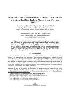
Multidisciplinary design optimization (MDO) studies the theory and application of numerical optimization techniques to the design of engineering systems involving multiple disciplines or components. Aircraft are prime examples of multidisciplinary systems, so it is no coincidence that MDO emerged within the aerospace research community. MDO originated in the late 1970s (Haftka, 1977; Haftka and Shore, 1979), following the successful application of numerical optimization to structural design in the 1960s (Schmit, 1960; Schmit Jr., 1981). Aircraft design was one of the first applications of MDO because there is much to be gained by simultaneously considering the various disciplines involved. One of the first applications of MDO was aircraft wing design, where aerodynamics, structures, and controls are strongly coupled disciplines (Ashley, 1982; Green, 1987; Grossman et al., 1988, 1990; Jansen et al., 2010; Kenway and Martins, 2014). MDO has since been extended to include aircraft sizing (Kroo et al., 1994; Wakayama, 1998) and has been applied to a wide range of other engineering systems (Martins and Lambe, 2013). One crucial aspect to consider in MDO is how to organize the coupling and optimization of the various disciplines involved. Research on the options for this organization has lead to the development of various MDO architectures (Martins and Lambe, 2013). MDO architectures can be either monolithic or distributed. In a monolithic approach, a single optimization problem is solved. In a distributed approach, the same problem is partitioned into multiple subproblems involving smaller subsets of the variables and constraints. In spite of numerous efforts, distributed architectures have been unable to outperform monolithic architectures in terms of convergence rate (Tedford and Martins, 2010). In aircraft design optimization problems, the objective and constraint functions are usually nonlinear, and thus a general purpose nonlinear optimizer that can handle constraints is required. There are two main classes of optimization algorithms: gradient-based and gradient-free (or derivative-free) algorithms. Gradient-free algorithms require only the values of the objective and constraint functions, while gradient-based algorithms, also require the gradients of these functions with respect to the design variables. Gradient-based methods utilize the gradient information to find the most promising directions in the design variable space, and converge to the optimum more quickly. This is especially true for problems with large numbers of design variables. Fig. 1 illustrates this by plotting the number of function evaluations required to minimized a multidimensional Rosenbrock function subject to nonlinear constraints. The number of function evaluation for the gradient-free optimizers (ALPSO, NSGA2) scale exponentially, and it becomes infeasible to perform optimization with respect to O(102 ) design variables or more using this type of algorithms. On the other hand, the gradient-based algorithms (SNOPT, SLSQP) scale much better, exhibiting linear convergence or better depending on the method used to compute the gradients. As we can see, computing the derivatives analytically makes a big difference in the performance. Thus, computing derivatives accurately and efficiently is essential for effective gradient-based optimization. The various methods for computing derivatives are described in Section 2. One of the issues with gradient-based optimizers is that they are based on the assumption that the functions involved are continuous and differentiable. In practice, a few discontinuities or non-differentiable points do not impede a gradient-based optimizer from converging to a minimum, unless the discontinuity is at a minimum itself. Another issue often cited
2
NSGA2
Quadratic
1e7 Number of evaluations
ALPSO
1e5
SLSQP-FD SNOPT-FD Linear SLSQP-AN
1e3
SNOPT-AN 1e1 1
4 16 64 Number of design variables
256
Figure 1: Computational cost of minimizing a constrained multidimensional Rosenbrock function with respect to the number of design variables. The gradient-free optimizers (ALPSO, NSGA2) scale exponentially, while the gradient-based optimizers (SNOPT, SLSQP) scale linearly with finite-difference derivatives (FD), and better than linearly with analytic derivatives (AN). with gradient-based optimization is that it converges to only one local minimum. While this is true, there is no optimization algorithm that is guaranteed to find the global minimum of a general non-convex function. Some gradient-free algorithms (including the two benchmarked in Fig. 1) do a wider exploration of the design space, which might find a better local minimum and even the global minimum. However, gradient-free algorithms require large numbers of function evaluations, and the computational cost becomes intractable for O(102 ) design variables or more. In the author’s experience, the existence of multiple local minima (multimodality) has been overstated. In aerodynamic shape optimization, for example, we tried to find multiple local minima, but we were unsuccessful (Lyu et al., 2015). We have had similar experience in other aircraft design and engineering systems optimization problems. Given the facts above, it is clear that our only hope for solving large-scale aircraft design optimization problems—problems with O(102 ) design variables or more—is to use a gradientbased optimization. One of the main challenges we tackle in these these lectures is to develop methods for computing gradients as accurately and efficiently as possible. Computing the derivatives of systems where multiple disciplines are coupled introduces another dimension to this challenge. In the next section of this lecture, we start by introducing the various methods for computing derivatives. Then, we unify these methods in Section 3 using a single equation: the unifying chain rule. This unification leads to a new framework for solving the state of multidisciplinary systems and their derivatives, which we describe in Section 4. To demonstrate this new strategy, we use it in an aircraft application in Section 5, where the mission profile,
3
airline allocation, and aircraft design are simultaneously optimized. In Part 2 of this lecture, we develop a framework for the MDO of aircraft configurations based on high-fidelity models, with emphasis on the coupling of the aerodynamics and structures disciplines. This leads to results in the aerostructural design optimization of flexible wings, which we discuss in detail.
2
Methods for computing derivatives
Derivatives play a central role in several numerical algorithms, such as Newton–Krylov methods applied to the solution of the PDEs. In the context of this lecture, we are particularly interested in computing derivatives to inform gradient-based optimization algorithms. The accuracy of the derivative computation affects the convergence behavior of the solver used in the algorithm. In the case of gradient-based optimization, accurate derivatives are important to ensure robust and efficient convergence, especially for problems with large numbers of design variables and constraints. The precision of the gradients limits how close we can get to the optimum solution, and inaccurate gradients can cause the optimizer to halt or to take a less direct route to the optimum that requires more iterations. To solve an optimization problem, a gradient-based algorithm requires the derivatives of the objective function with respect to each design variable, and the derivatives of all the constraints with respect to the design variables. In general, we need to compute the derivatives vector-valued function f with respect to a vector of independent variables x, which yields a Jacobian matrix,
df1 dx1 df . = .. dx dfnf dx1
··· ..
.
···
df1 dxnx .. , . dfnf dxnx
(1)
which is an nf × nx matrix. 2.1 Finite differences Finite-difference methods are widely used to compute derivatives due to their simplicity and the fact that they can be implemented even when a the function evaluation is provided as black box. Finite-difference formulas are derived by combining Taylor series expansions. Using the right combinations of these expansions, it is possible to obtain finite-difference formulas that estimate an arbitrary order derivative with any required order truncation error. The simplest finite-difference formula can be directly derived from one Taylor series expansion, yielding df f (x + ej h) − f (x) = + O(h), (2) dxj h where h is a small perturbation and ej is a vector of zeros with a unity entry in row j. This formula requires the evaluation of the model at the reference point x and one perturbed point x+ej h, and yields one column of the Jacobian (1). Each additional column requires an additional evaluation of the computational model. Hence, the cost of computing the complete 4
Jacobian is proportional to the number of input variables, nx . When the computational model is nonlinear, the constant of proportionality with respect to the number of variables can be less than one if the solutions for the successive steps are warm-started with the previous solution. Estimating derivatives using finite-difference formulas is subject to the step-size dilemma: we want to reduce the truncation error by reducing h but below a certain value of h, errors due to subtractive cancellation become dominant, and for small enough h, the finite-different formula just yields zero. Most gradient-based optimizers use finite-differences by default to compute the gradients. For problems with large numbers of design variables, the computation of the derivatives usually becomes the bottleneck in the optimization cycle. In addition, inaccuracies in the derivatives due to subtractive cancellation are often the culprit in cases where gradient-based optimizers fail to converge. Therefore, we need methods that are both more accurate and efficient. 2.2 Complex-step method The complex-step derivative approximation computes derivatives of real functions using complex variables. This method originated with the work of Lyness and Moler (1967). They developed several methods that made use of complex variables, including a reliable method for calculating the nth derivative of an analytic function. This technique was rediscovered by Squire and Trapp (1998), who derived a simple formula for estimating the first derivative. This estimate is very accurate, extremely robust, and easy to implement (Martins et al., 2003). The first application of this approach to an iterative solver was by Anderson et al. (2001), who used it to compute derivatives of a Navier–Stokes solver, and later multidisciplinary systems (Newman III et al., 2003). Martins et al. (2003) showed that the complex-step method is generally applicable to any computer program and described the detailed procedure for its implementation. They also presented an alternative way of deriving and understanding the complex step, and connect this to automatic differentiation (explained in Section 2.3). The complex-step method requires access to the source code. Martins et al. (2003) provide a script that facilitates the implementation of the complex-step method to Fortran codes, and explain how to implement this method in Matlab, C/C++, and Python. The cost of computing a gradient using the complex-step, like finite differences, is proportional to the number of design variables, so it is not recommended for large-scale optimization. However, the complex-step approach has been extremely useful in the verification of high-fidelity aerodynamic (Lyu et al., 2013; Mader et al., 2008) and aerostructural derivatives (Kenway et al., 2014; Martins et al., 2005). The complex-step method is now widely used, with applications not only in engineering, but in the natural sciences as well. The complex-step derivative approximation, like finite-difference formulas, can also be derived using a Taylor series expansion. Rather than using a real step h, we now use a pure imaginary step, ih. If f is a real function in real variables and it is also analytic, we can expand it in a Taylor series about a real point x as follows: h2 d2 f ih3 d3 f df − − + ... f (x + ihej ) = f (x) + ih dxj 2 dx2j 6 dx3j 5
(3)
Taking the imaginary parts of both sides of this equation and dividing it by h yields Im [f (x + ihej )] df = + O(h2 ), dxj h
(4)
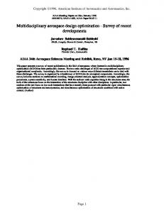
Because there is no subtraction operation in the complex-step derivative approximation (4), the only source of numerical error is the O(h2 ) truncation error. By decreasing h to a small enough value, we can ensure that the truncation error is of the same order as the numerical precision of the evaluation of f . To show the how the complex-step method works, we consider an analytic function for which the derivative was computed to 16 digits and then compared the relative error of the complex-step approximation (4) to that of the forward finite-difference (2). As we can see in Fig. 2, the forward-difference estimate initially converges to the exact result at a linear rate since its truncation error is O(h). However, as the step is reduced below a value of about 10−8 , the subtractive cancellation error becomes significant and the estimates are unreliable. When the interval h is so small that no difference exists in the output (for steps smaller than 10−16 ) the finite-difference estimates eventually yields zero and then the relative error is 1. Comparing the best accuracy of each of these approaches, we can see that by using finite-difference we only achieve a fraction of the accuracy that is obtained by using the complex-step approximation. 102 100
Log of relative error
10-2 10-4 10-6 10-8 10-10 10-12 10-14
FD CS
10-16 10-18 -20 10 10-18 10-16 10-14 10-12 10-10 10-8 Log of step size
10-6
10-4
10-2
100
Figure 2: Relative error in the derivative estimate versus step size.
2.3 Automatic differentiation Symbolic differentiation is another option for computing derivatives. One can differentiate explicit mathematical expressions by hand or by using symbolic differentiation software. However, many engineering models cannot written explicitly in closed form, relying instead 6
on iterative numerical procedures expressed as computer programs. Automatic differentiation (AD)—also known as algorithmic differentiation—is based on the systematic symbolic differentiation of each line of a computer program, and the accumulation of total derivatives using the chain rule. The method relies on tools that automatically produce a program that computes user-specified derivatives based on the original program (Griewank, 2000). When using AD, we consider all variables assigned in a computer program, t = [t1 , t2 , . . . , tm ] We consider the first n variables in this set to be independent variables t1 , t2 , . . . , tn , which for our purposes are the design variables, x. We also need to consider the dependent variables, tn+1 , tn+2 , . . . , tm . These are all the intermediate variables in the algorithm, including the outputs, f , which are the functions we want to differentiate. We can then write the sequence of operations in any algorithm as ti = Ti (t1 , t2 , . . . ti−1 ) ,
i = n + 1, n + 2, . . . , m.
(5)
The chain rule can be applied to each of these operations and can be written as i−1 X ∂Ti ∂tk dti = δij + . dtj k=j ∂tk ∂tj
(6)
Using the forward mode, we choose one j and keep it fixed. We then work our way forward in the index i until we get the desired derivative. The reverse mode, on the other hand, works by fixing i to the index of the quantity we want to differentiate, and working our way backwards in the index j all the way down to the independent variables. There are two main ways of implementing automatic differentiation: source code transformation and operator overloading. Tools that use source code transformation add new statements to the original source code that compute the derivatives of the original statements. The operator overloading approach consists in defining a new user-defined type that is used instead of real numbers. This new type includes not only the value of the original variable, but its derivative as well. All intrinsic operations and functions have to be redefined (overloaded) to compute the derivatives together with the original computations. The operator overloading approach results in fewer changes to the original code, but is usually less efficient (Griewank, 2000; Pryce and Reid, 1998). There are automatic differentiation tools available for a variety of programming languages including C/C++, and Fortran (Carle and Fagan, 2000; Giering and Kaminski, 2002; Gockenbach, 2000; Hascoët and Pascual, 2004; Pascual and Hascoët, 2005). 2.4 Analytic methods Analytic methods are based on the linearization of the numerical model equations. Like AD, the numerical precision of analytic methods is the same as that of the original algorithm. In addition, analytic methods are usually more efficient than AD for a given problem. However, analytic methods are much more involved than the other methods, since they require detailed knowledge of the computational model and a long implementation time. Analytic methods are applicable when we have a quantity of interest f that depends implicitly on the independent variables of interest x as follows f = F (x, y(x)). 7
(7)
The implicit relationship between the state variables y and the independent variables is defined by the solution of a set of governing equations that can be written as residuals, r = R(x, y(x)) = 0.
(8)
By writing the computational model in this form, we have assumed a discrete analytic approach. This is in contrast to the continuous approach, in which the equations are differentiated before being discretized. We do not discuss the continuous approach in this lecture, but ample literature can be found on the subject (Anderson Jr., 1999; Giles and Pierce, 2000; Jameson, 1988; Liu and Canfield, 2012; Sirkes and Tziperman, 1997), including discussions comparing the two approaches (Dwight and Brezillon, 2006; Nadarajah and Jameson, 2000; Peter and Dwight, 2010). As a first step toward obtaining the derivatives that we want to compute, we use the chain rule to write the total derivative of f as ∂F ∂F dy df = + , dx ∂x ∂y dx
(9)
where the result is an nf × nx Jacobian matrix. It is important to distinguish the total and partial derivatives and define their context. The partial derivatives represent the variation of f = F (x) with respect to changes in x for a fixed y, while the total derivative df / dx takes into account the change in y that is required to keep the residual equations (8) equal to zero. Since the governing equations must always be satisfied, the total derivative of the residuals (8) with respect to the design variables must also be zero. Thus, using the chain rule we obtain ∂R ∂R dy dr = + = 0. (10) dx ∂x ∂y dx The partial derivatives in Eqs. (9) and (10) can be computed using the methods described earlier (finite differences, complex step, and AD). The computation of the total derivative matrix dy/ dx has a much higher computational cost than any of the partial derivatives, since it requires the solution of the residual equations (8). Rearranging the linearized residual equations (10) we can compute the total derivative matrix dy/ dx by solving the linear system, ∂R dy ∂R =− . (11) ∂y dx ∂x Substituting this result into the total derivative equation (9), we obtain dy − dx
z "
df ∂F ∂F ∂R = − dx ∂x ∂y ∂y |
{z ψ
}| #−1
{
∂R . ∂x
(12)
}
The inverse of the square Jacobian matrix ∂R/∂y is not necessarily calculated explicitly. We use the inverse to denote that this matrix needs to be solved as a linear system with some right-hand-side vector. Equation (12) shows that there are two ways of obtaining the total derivative matrix dy/ dx, depending on which right-hand side is chosen for the solution of the linear system. 8
2.4.1 Direct method The direct method involves solving the linear system with −∂R/∂x as the right-hand side vector, which results in the linear system (11). This linear system needs to be solved for nx right-hand sides to get the full Jacobian matrix dy/ dx. Then, we can use dy/ dx in Eq. (9) to obtain the derivatives of interest, df / dx. As in the case of finite differences, the cost of computing derivatives with the direct method is proportional to the number of design variables, nx . In a case where the computational model is a nonlinear system, the direct method can be advantageous. Both methods require the solution of a system of the same size nx times, but the direct method just solves the linear system (11), while the finite-difference method solves the original nonlinear system (8). Even though the various solutions required for the finite-difference method can be warm-started from a previous solution, a nonlinear solution typically requires multiple iterations to converge. The direct method is even more advantageous when a factorization of ∂R/∂y is available, since each solution of the linear system would then consist in an inexpensive back substitution. 2.4.2 Adjoint method Adjoint methods for computing derivatives have been known and used for over three decades. They were first applied to solve optimal control problems and thereafter used to perform sensitivity analysis of linear structural finite element models. The first application to fluid dynamics is due to Pironneau (1974). The method was then extended by Jameson (1988) to perform airfoil shape optimization, and later applied to three-dimensional problems, leading to aerodynamic shape optimization of complete aircraft configurations (Lyu and Martins, 2013; Reuther et al., 1999a,b; Vassberg and Jameson, 2002) and shape optimization considering both aerodynamics and structures (Kenway et al., 2012; Martins et al., 2004). The adjoint method has since been generalized for multidisciplinary systems (Martins and Hwang, 2013). The adjoint equation is encapsulated in the total derivative equation (12), where we observe that there is an alternative option for computing the total derivatives: the linear system involving the large square Jacobian matrix ∂R/∂y can be solved with ∂f /∂y as the right-hand side. This results in the adjoint equations, "
∂R ∂y
#T
"
∂F ψ=− ∂y
#T
,
(13)
which is a linear systems where ψ is the adjoint matrix (of size ny × nf ). Although this is usually expressed as a vector, we obtain a matrix due to our generalization for the case where f is a vector. This linear system needs to be solved for each column of [∂F /∂y]T , and thus the computational cost is proportional to the number of quantities of interest, nf . The adjoint vector can then be substituted into Eq. (12) to find the total derivative, df ∂F ∂R = + ψT . (14) dx ∂x ∂x Thus, the cost of computing the Jacobian ∂f /∂x using the adjoint method is independent of the number of design variables, nx , and instead it is proportional to the number of quantities of interest, nf . 9
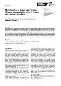
As previously mentioned, the partial derivatives shown in these equations need to be computed using some other method. They can be differentiated symbolically or computed by finite differences, the complex-step method, or even AD. The use of AD to automatically produce the code that computes these partials derivatives has shown to be particularly effective in the development of analytic methods for PDE solvers (Lyu et al., 2013; Mader et al., 2008). More detail on this technique is provided in Part 2 of this lecture. By comparing the direct and adjoint method, we also notice that all the partial derivative terms that need to be computed are identical, and that the difference in their relative cost comes only from the choice of which right-hand side to use with the residual Jacobian. Figure 3 shows the sizes of the matrices in Eq. (12), which depend on the shape of df / dx. These diagrams illustrate why the direct method is preferable when nx < nf and the adjoint method is more efficient when nx > nf . From forward chain rule I 0 0 I ∂ R ∂ R dy I − − 0 = 0 ∂x ∂y dx ∂ F ∂ F df 0 − − I dx ∂x ∂y
Solution
df ∂F ∂F = − dx ∂x ∂y
�
∂R ∂y
�−1
From reverse chain rule ∂ RT ∂ F T df T I− − 0 ∂x T ∂x T dx df T = 0 0− ∂ R − ∂ F I ∂y ∂y dr I 0 0 I
∂R ∂x
= −
=
= nx < nf
= =
−
=
nx > n f Direct method df ∂F ∂ F dy = + dx ∂x ∂y dx
= + =
+
−
Adjoint method ∂ R dy ∂R = ∂y dx ∂x
−
df ∂F df ∂ R = + dx ∂x dr ∂x
=
nx < nf
=
nx > nf
= + =
−
+
−
∂ RT df T ∂F T = ∂y dr ∂y
− −
= =
Figure 3: Block matrix diagrams illustrating the structure of the direct and adjoint equations, assuming that ny � nx , nf . The blue matrices consist of partial derivatives, which are relatively cheap to compute, and the red matrices consist of the total derivatives computed by solving the linear systems.
3
Unified mathematical formulation
In this sections, we derive an equation based on the chain rule of differentiation that unifies all the methods described in Section 2, which inspired a new perspective on the mathematical formulation of systems with multiple numerical models. This new perspective leads to the hierarchical strategy for solving multidisciplinary systems and for computing the derivatives 10
of these systems that we describe in Section 4. In our formulation, we use the term numerical model to refer to the discrete variables and their explicit or implicit definitions, whereas computational model refers to the code that implements the numerical model. Section 3.1 describes the notation for any general numerical model, Sec. 3.2 formulates the general numerical model as a single system of algebraic equations, and in Sec. 3.3 we show how the derivatives of the coupled system are computed. 3.1 Notation For our purposes, a variable represents a vector of a single type of physical or abstract quantity in a numerical model. In many settings, each individual scalar is referred to as a separate variable; however, in the current context, a group of scalars representing the same quantity—such as a vector comprised of temperature values at different time instances—is collectively referred to as a single variable. The only exception is for the design variables: We call each scalar varied by the optimizer a separate design variable, to remain consistent with the terminology used in the optimization literature. Fundamentally, numerical models capture the relationships between quantities, i.e., the response of one or more quantities to independent changes in other quantities. Thus, it is useful to classify the variables in a numerical model as either input, state, or output variables. Input variables are independent variables whose values are set externally by either the designer or the optimizer, so the design variables (x) for an optimization problem are a subset of the input variables. Output variables are the dependent variables of interest, computed explicitly as a function of the input and state variables, and the output variables contain the objective and constraints in an optimization problem (f ). State variables (y) are dependent variables computed by the model (8) in the process of computing the output variables, and they are defined by implicit or explicit functions of the design variables and other state variables. Using this nomenclature, a numerical model can be expressed as: y1 = Y1 (x1 , . . . , xm , y2 , . . . , yp ), .. . yp = Yp (x1 , . . . , xm , y1 , . . . , yp−1 ),
(15)
f1 = F1 (x1 , . . . , xm , y1 , . . . , yp ), .. . fp = Fp (x1 , . . . , xm , y1 , . . . , yp ), where some of the state variables also have a residual function Rk associated with them. 3.2 Monolithic formulation We now reformulate the numerical model (15) as a single system of algebraic equations. We assume that x∗k is the value of input variable xk for all k = 1, . . . , m, at the point at which the numerical model is being evaluated. The first step is to concatenate the set of input,
11
state and output variables into a single vector, u = (u1 , . . . , un )T = (x1 , . . . , xm , y1 , . . . , yp , f1 , . . . , fq )T ,
(16)
where n = m + p + q. The corresponding residuals are given by, R1 (u) = x1 − x∗1 , .. . Rm (u) = xm(− x∗m , y1 − Y1 (x1 , . . . , xm , y2 , . . . , yp ) , y1 is explicitly defined Rm+1 (u) = , −R1 (x1 , . . . , xm , y1 , . . . , yp ) , y1 is implicitly defined .. .
(17)
(
yp − Yp (x1 , . . . , xm , y1 , . . . , yp−1 ) , yp is explicitly defined , −Rp (x1 , . . . , xm , y1 , . . . , yp ) , yp is implicitly defined Rm+p+1 (u) = f1 − F1 (x1 , . . . , xm , y1 , . . . , yp ), .. . Rm+p (u) =
Rm+p+q (u) = fq − Fq (x1 , . . . , xm , y1 , . . . , yp ). The numerical model can be written more compactly as,
R1 (u1 , . . . , un ) = 0 .. ⇔ R(u) = 0. . Rn (u1 , . . . , un ) = 0
(18)
The unified formulation of a numerical model is the algebraic system of equations R(u) = 0, which we call the fundamental system. Its significance lies in the fact that the vector u∗ that solves the fundamental system (18) satisfies the numerical model (15). 3.3 Derivative computation In the context of optimization, the design variables that the optimizer varies are a subset of the input variables of the numerical model, and the objective and constraint functions given to the optimizer are a subset of the output variables of the numerical model. Thus, the derivatives of interest are a subset of the derivatives of the output variables with respect to the input variables. Starting from the fundamental system (18), we can derive an equation that unifies all four methods described in Sec. 2. As we will see, each method is determined the choice of the state variables—on one extreme, including no state variables in the vector u results in a finite-step method and on the other extreme, including the variables from every line of code in a computational model results in automatic differentiation (Martins and Hwang, 2013). To obtain the analytic methods of Sec. 2.4, the fundamental system must be defined with the original residual used for each implicit state variable. For the explicit state variables, the residuals are defined as the value of the state variables minus the output of the explicit
12
function. We begin by defining
x1 . x = .. , xm
y1 . y = .. , yp
f1 . f = .. fq
(19)
as the input, state, and output vectors and defining the respective functions,
Y1 . Y = .. , Yp
F1 . F = .. Fq
(20)
Then, the fundamental system has the form,
x u = y f
x − x∗ and R(u) = −R(x, y) , f − F (x, y)
(21)
and the numerical model is encapsulated in the function, G : x 7→ F (x, Y (x)),
(22)
which maps the inputs x to the outputs f . The derivatives of interest are ∂G/∂x. The following proposition shows how ∂G/∂x can be computed from the fundamental system defined by Eq. (21). Proposition 1. Let R and u be as defined by Eq. inverse is defined as xx A Axy −1 ∂R yx Ayy = A ∂u Af x Af y
(21). If ∂R/∂u is invertible and the Axf Ayf , Af f
(23)
then the derivatives we seek are in the bottom left block in this Jacobian, i.e., ∂G = Af x , ∂x ∗ where ∂R/∂u is evaluated at u satisfying R(u∗ ) = 0.
(24)
Proof. By construction, we have I 0 0 xx ∂R A Axy Axf I 0 0 −1 ∂R ∂R ∂(R ) yx − − 0 Ayy Ayf = I =⇒ = 0 I 0 . ∂x A ∂x ∂u ∂r ∂F Af x Af y Af f ∂F 0 0 I − − I ∂x ∂x Block-forward substitution for the first block-column yields
(25)
I xx A ∂R −1 ∂R − yx . A = ∂y ∂x −1 fx A ∂F ∂F ∂R ∂R − ∂x ∂y ∂y ∂x 13
(26)
Now, G is a composition of functions mapping x 7→ (x, Y (x)) and (x, y) 7→ F (x, y), so applying the chain rule yields "
∂F ∂G = ∂x ∂x
∂F I ∂Y . ∂y ∂x #
(27)
Since ∂R/∂y is invertible, the implicit function theorem states ∂Y ∂R −1 ∂R =− . ∂x ∂y ∂x
(28)
Combining the two equations above yields ∂G ∂F ∂F ∂R −1 ∂R = − . ∂x ∂x ∂y ∂y ∂x
(29)
∂G = Af x , ∂x
(30)
Therefore,
as required. The application of the inverse function theorem explains why the lower left nf × nx block of ∂R/∂u is equal to the Jacobian with the derivatives of interest that we denoted in Sec. 2 as df / dx. Assuming ∂R/∂u is invertible, the inverse function theorem guarantees the existence of a locally defined inverse function R−1 : r 7→ u|R(u) = r that satisfies ∂(R−1 ) ∂R = ∂r ∂u "
#−1
.
(31)
The concept of a total derivative is used in many settings, but it is difficult to find a clear definition in the literature—they are usually defined in terms of other total derivatives as in Eq. (12). Total derivatives are useful for distinguishing direct and indirect dependence on a variable. In the total derivative (12), df / dx captures both the explicit dependence of F on the argument x and the indirect dependence via other arguments of F (y in this case) that depend on x. The Jacobian ∂(R−1 )/∂r captures a similar relationship because the (i, j)th entry of the matrix ∂(R−1 )/∂r captures the dependence of the ith component of u on the jth component of r both explicitly and indirectly via the other components of u. This motivates the following definition of the total derivative. Definition 1. Given the algebraic system of equations R(u) = 0, assume ∂R/∂u is invertible at the solution of this system. The matrix of total derivatives du/dr is defined to be du ∂(R−1 ) = , dr ∂r where ∂(R−1 )/∂r is evaluated at r = 0. 14
(32)
Following from Eq. (31), the matrix du/ dr is also equal to the inverse of ∂R/∂u, leading to
∂R T du T ∂R du =I= , (33) ∂u dr ∂u dr which we refer to as the unifying chain rule equation. The structure of the left inequality in this equation is shown in Fig. 4. The left and right equalities are denoted as the forward mode and the reverse mode, respectively, drawing inspiration from terminology used in AD (Sec. 2.3). The unifying chain rule (33) was first presented by Martins and Hwang (2013) with different notation and derivation. In that paper, we also show how this equation unifies all methods—how the finite-difference method, complex-step method, AD, direct method, adjoint method, and the chain rule can all be derived from the unifying chain rule (33). Basically, we can derive the equations for the different methods from the unifying chain rule (33) by the appropriate definition of R and u. In the extreme case of the finite-difference or complex-step methods, u is simply the concatenation of the inputs x and outputs f . In the other end of the spectrum, defining u as every single value in a computer program yields AD (Martins and Hwang, 2013). For the independent variables, the r in the denominator of du/ dr can be replaced with the symbol for the variable itself, as shown in Fig. 4. The derivatives of interest are df / dx, which is a sub-block of du/ dr. Computing df / dx involves solving a linear system with multiple right-hand sides, so this is more efficient with the left or right equality in Eq. (33), depending on the relative sizes of f and x.
I
0
0
I
0
0
−
∂R ∂x
−
∂R ∂y
0
dy dx
dy dr
0
−
∂F ∂x
−
∂F ∂y
I
df dx
df dr
I
=
I
0
0
0
I
0
0
0
I
Figure 4: Block structure of the matrices in the left equality of Eq. (33).
4
Hierarchical solution strategy
The unifying chain rule (33) applies to multidisciplinary systems (where R and u contain multiple sets of sub-vectors), and leads to the modular analysis and unified derivatives (MAUD) MDO architecture. The high-level objective of the MAUD architecture is to facilitate two tasks: the evaluation of a computational model with multiple components and the efficient computation of its derivatives across the various components. The significance of the mathematical formulation presented in Sec. 3 is that the different algorithms for performing these
15
two tasks are unified in an elegant way that simplifies the implementation of the computational framework. The task of evaluating a coupled computational model reduces to solving a system of algebraic equations, and the task of computing derivatives reduces to solving a system of linear equations. At the highest level, the MAUD solves four types of systems: 1. The nonlinear system
2. The Newton system
3. Derivatives in forward mode
4. Derivatives in reverse mode
∂R du ∂R T du T ∂R ∆u = −r =I =I ∂u ∂u dr ∂u dr The MAUD architecture is designed to handle components with distributed data parallelism. This means that a problem in MAUD is not necessarily a single system of equations. Such a monolithic system could result in a significant memory and computational time overhead. For example, if a computational model has two components that can be run in sequence because the second component does not influence the first one, it would be more efficient to run a block Gauss–Seidel iteration over the two components rather than using a Krylov solver for the whole system. Fig. 5 shows several problems with unique structures that MAUD is able to exploit. To exploit problem structure, the MAUD architecture performs a recursive hierarchical algorithm for solving the nonlinear and linear systems. MAUD also adopts a matrix-free approach, since it uses only nonlinear and linear operations on vectors. R(u) = 0
16
x
x
x
y1a
y1a y1
y1b
y1b
y2a
y2a y2
y2a
y2a f
Serial · Parallel
Serial · Parallel · Serial
x
f
f
x
Serial · Parallel · Coupled
x y1a
y1a
y1 y1b
y1b y2a
y2a
y2 y2a f
Serial · Coupled
y2a f
Serial · Coupled · Serial
f
Serial · Coupled · Parallel
Figure 5: MAUD exploits the structure of multidisciplinary systems by using assemblies of serial, parallel, and coupled solution solvers.
17
This section describes the MAUD hierarchical solution strategy. Section 4.1 begins by presenting the hierarchical decomposition of the fundamental system (18) into smaller systems of algebraic equations. Section 4.2 presents the MAUD hierarchical decomposition algorithm, and Sec. 4.3 presents the design of MAUD’s data structures. 4.1 Mathematical decomposition To solve the fundamental system (18) efficiently, we partition the global unknown vector and system of equations into smaller sets. This partitioning is recursive for additional flexibility in handling complex multidisciplinary systems, resulting in a hierarchical decomposition of the fundamental system (18). We introduce a smaller algebraic system, an intermediate system, that selects a subset of the fundamental system residuals and unknowns. We define the index set S = {i + 1, . . . , j},
0 ≤ i < j ≤ n,
(34)
to represent the indices of the variables that make up the unknowns for this smaller algebraic system. The residual function for this intermediate system is RS : D1 × · · · × Dn → RNi+1 × · · · × RNj ,
(35)
formed by concatenating the residual functions corresponding to the indices in S. Let pS = (u1 , . . . , ui , uj+1 , . . . , un ) and uS = (ui+1 , . . . , uj ) partition u into the parameter vector and unknown vector, respectively. Then, the intermediate system for index set S implicitly defines uS as a function of pS : Ri+1 (u1 , . . . , ui , ui+1 , . . . , uj , uj+1 , . . . , un ) = 0 .. ⇔ RS (pS , uS ) = 0. . Rj (u1 , . . . , ui , ui+1 , . . . , uj , uj+1 , . . . , un ) = 0
|
{z
pS
} |
{z
uS
} |
{z
pS
(36)
}
The significance of this definition is that intermediate systems are formulated and solved in the process of solving the fundamental system. Solving an intermediate system that owns only one variable or a group of related variables in its unknown vector is analogous to executing a component in the traditional view of MDO—that is, computing the component’s outputs given the values of the inputs, which are contained in pS in this case. However, this formulation allows the definition of intermediate systems that group together other intermediate systems that may correspond to components, and overall, this enables a hierarchical decomposition of all the variables in the computational model. 4.2 Solution algorithm We now present the hierarchical solution algorithm at the core of the MAUD architecture. The fundamental system owns the full set of n variables in the numerical model at the hierarchy tree root level. The fundamental system contains a group of intermediate systems that together partition the n variables and form the second level of the hierarchy tree. Each of these intermediate systems can contain other intermediate systems, and so on, until we 18
reach the leaves of the hierarchy tree, i.e., intermediate systems that do not contain other intermediate systems. MAUD enables a small and simple interface that captures all operations required from any intermediate system. Thus, an intermediate system defined by an index set S is given by RS (pS , uS ) = 0, (37) where uS is the unknown vector, pS is the parameter vector, and RS is the residual function. We assume that there is an implicit function that computes the unknown vector in terms of the parameter vector. Therefore, we can view pS as the inputs and uS as the outputs of this system. For a given intermediate system RS (pS , uS ) = 0, the interface consists of the following operations (where we omit the subscript S for brevity): apply_nonlinear: (p, u) 7→ r = R(p, u). This operation computes the residual functions for the current intermediate system. It is used to compute the right-hand side of the linear system in Newton’s method and to check the convergence of the current intermediate system. solve_nonlinear: p 7→ u. This operation solves R(p, u) = 0 inexactly or to the required convergence tolerance. It is optional to implement this method, since Newton’s method is used when the user does not provide a custom solver. ∂R ∂R dp + du, forward mode ∂p ∂u ! apply_linear: ∂R T ∂R T dr, du = dr , reverse mode. dr 7→ dp = ∂p ∂u This operation allows the component to implicitly provide Jacobians ∂R/∂(p, u)to MAUD’s solver. By implementing this as a linear operator, the user does not need to specify how each component stores or computes the Jacobian. This constitutes a single, simple interface that can handle sparse of dense Jacobians, as well as Jacobianfree components. Either the forward or reverse modes can be used for computing the derivatives.
solve_linear:
(dp, du) 7→ dr =
∂R du = dr , (dr) 7→ du ∂uT ∂R (du) 7→ dr dr = du , ∂u
forward mode reverse mode.
This operation implements the inverse of ∂R/∂u as a linear operator. Like solve_nonlinear, it is optional, since the framework uses a Krylov iterative solver if apply_linear is known. linearize: This operation is part of the interface because many problems require an initial assembly (and in some cases factorization) of the Jacobian, and repeated applications of the matrix or factorization have a substantially lower cost.
19
The software design for this hierarchical algorithm is naturally object-oriented, with an instance of a System class created for each intermediate system. The lowest-level intermediate systems—the leaves in the tree—are instances of the ElementarySystem class, while all other intermediate systems are instances of the CompoundSystem class, because they contain other System instances. In other words, the ElementarySystem objects are grouped together by CompoundSystem objects, which can in turn be grouped by other CompoundSystem objects. Figure 6 illustrates the containment relationships between the ElementarySystem class, CompoundSystem class, and variables for a general computational model. CompoundSystem
CompoundSystem
CompoundSystem
ElementarySystem
Variable
CompoundSystem
ElementarySystem
Variable
Variable
Variable
Figure 6: Class containment diagram showing the relationships between objects in a computational model implemented in the MAUD architecture. The ElementarySystem and CompoundSystem classes inherit from a base System class. The ElementarySystem class has three derived classes, reflecting whether the system contains independent, explicitly defined, or implicitly defined variables. The user implements each component in MAUD as a class inheriting from one of these three classes and directly implements operations such as computing the residual function value. Each component contains a subset of the variables, which form the unknown vector in the component’s intermediate system. During initialization, the ElementarySystem object must declare its variables as well as its arguments—external variables that depend on the ElementarySystem variables. In contrast, the CompoundSystem class is meant to group other System objects together, so their operations recursively call those of their children. Moreover, they perform transfer of data potentially distributed across multiple processors. The CompoundSystem class has two derived classes that handle parallelism in different ways. In the hierarchy tree in Fig. 6, the root CompoundSystem is stored and run on all processors running the job. If a given system object is a SerialSystem, it passes all of its processors to the System objects it contains and runs its recursive operations sequentially among the contained systems. If a system object is a ParallelSystem, it partitions its group of processors among the System objects it contains and runs its recursive operations concurrently among the contained systems. The same applies to all CompoundSystem objects, and in this manner, each System object is assigned a subset of or all of its containing System object’s processors. The MAUD class inheritance diagram is shown in Fig. 7. This object-oriented design allows all of MAUD’s 20
System
ElementarySystem
IndependentSystem
ExplicitSystem
CompoundSystem
ImplicitSystem
SerialSystem
ParallelSystem
Figure 7: Class inheritance diagram showing the relationships between the System classes. built-in solvers to be implemented as methods of one of the base system classes. Table 1 shows the classes where each built-in solver is implemented. Table 1: MAUD’s’ four elementary operations and their implementations in each type of System class.
Virtual methods
System classes System
CompoundSystem
ElementarySystem
apply_nonlinear
—
Recursive
User-implemented
apply_linear
—
Recursive
User-implemented or FD∗
solve_nonlinear
Newton with
Nonlinear block
Optional
line search
Gauss–Seidel/Jacobi
Krylov-type with
Linear block
preconditioning
Gauss–Seidel/Jacobi
solve_linear
Optional
*FD: finite-difference approximation of the Jacobian.
4.3 Data structures Efficient data structures are necessary to avoid memory and computing overhead in problems with large numbers of unknowns. For each system, MAUD stores six vectors: u, p, and f for the nonlinear problem and du, dp, and df for the linear problem. The latter three can be interpreted as buffers that contain the data for the solution vector or the right-hand side vector, depending on the situation. Among these six vectors, u, du, f , and df are instances of the UnknownVec class, while p and dp are instances of the ParameterVec class. For the UnknownVec instances, data is shared with contained or containing systems; that is, the full u, du, f , and df vectors are allocated in the top-level CompoundSystem, and all other systems store pointers onto sub-vectors of the global vector. Compared to allocating separate vectors in each system, this approach saves memory as well as computation time, since the subsystems operate directly on sub-vectors of the larger system’s vector A
21
ParameterVec stores only the variables and components that an ElementarySystem declares. For illustration, Fig. 8 shows how the u and p vectors are stored. MAUD automates parallel data transfer between UnknownVec and ParameterVec instances. Legend
CompoundSystem
u, pointer
CompoundSystem
u, allocated
.. .
p, pointer
.. . CompoundSystem
p, allocated
ElementarySystem v1
···
vi1
vi1 +1
···
vi2
vi2 +1
···
vN
Variables
Data stored on processor k
Figure 8: Data storage for the u and p vectors for an ElementarySystem object and all of the CompoundSystem instances above it in the hierarchy tree.
4.4 Implementation A minimalistic framework based on the MAUD architecture has been implemented using the Python programming language. This implementation depends only on the NumPy package for handling local vectors and on the petsc4py package to use the portable, extensible toolkit for scientific computation (PETSc) (Balay et al., 1997). PETSc is used for all parallel data transfers, and its Krylov iterative methods are used as MAUD’s linear solvers, with flexible generalized minimal residual (fGMRES) as the default solver. The entire implementation is contained in a single Python file with about one thousand lines of code, thanks to the MAUD architecture’s monolithic mathematical formulation and the use of PETSc. The MAUD architecture has been adopted as the algorithmic core of NASA’s OpenMDAO framework (Gray et al., 2013). OpenMDAO is an open-source computational framework designed to facilitate the solution of multidisciplinary optimization problems. Since it uses MAUD, OpenMDAO provides coupled adjoint-based derivative computation, as one of its key features. The mission analysis and allocation models described in the next section have also been implemented in OpenMDAO.
5
Application to aircraft design
We now present an application of MAUD to the large-scale optimization of an aircraft configuration where the airline allocation, mission profile, and aircraft design are all optimized simultaneously. 5.1 Motivation Typically, when performing aircraft design optimization, only a limited number of flight conditions is considered. For instance, aerodynamic shape optimization using CFD might be run at a fixed, pre-determined set of lift coefficients that represent typical values of similarlysized aircraft during actual operation (Kenway and Martins, 2015). Similarly, aerostructural 22
optimization that couples CFD and FEA designs the aerodynamic shape and structural sizing simultaneously, while considering fuel burn for a limited number of flight conditions (Kenway and Martins, 2014; Liem et al., 2015). Herein we aim to widen the scope of the high-fidelity optimization to include some of the requirement-definition part of conceptual design. Instead of optimizing the aircraft design for a set of representative missions—or a design range, design Mach number, and payload—we let the algorithm choose on which routes in a network it is optimal to fly this next-generation aircraft, and which cruise Mach numbers are optimal on those routes. Thus, we view the problem from the airline’s perspective, since the airlines are the customers who define the requirements in the conceptual-design sense. With this formulation, the objective function is the profit margin for the airline. We assume an airline network—a set of routes that the airline operates—as well as a finite-sized fleet of existing and next-generation aircraft that the airline can deploy on those routes. The optimizer chooses how to allocate the fleet of aircraft, selects the optimal mission profile for each aircraft flying on each route, and designs the next-generation aircraft, all at the same time. Thus, we call this formulation allocation-mission-design optimization (AMD), since all three aspect are optimized simultaneously within a single problem. In this approach, the effective design range and payload for the next-generation aircraft is implicitly determined through optimization. The optimizer has the ability to design a smaller aircraft that is particularly efficient for short-range missions, or it could size the aircraft for long-range missions and cover the short-range routes for which it is over-designed using existing aircraft. This section presents the first implementation and solution of the AMD optimization problem (Hwang and Martins, 2016). For the design component, we do aerodynamic shape optimization based on 3D Euler CFD. In the mission component, we optimize the shape of the altitude profiles for each mission, and we also make the cruise Mach number for each mission a design variable with a linear Mach number variation during climb and descent. For the allocation, we consider a hypothetical 128-route network with fixed passenger demand on each route and a fleet consisting of 4 existing types of aircraft in addition to the simultaneous design of the next-generation aircraft. 5.2 Computational models The software components that are integrated to solve the AMD optimization problem include: a CFD mesh deformation algorithm, a CFD solver, a mission analysis model, an aircraft allocation model, and an optimizer. The CFD mesh deformation algorithm we use propagates the displacements and rotations from the deformed surface to the full CFD volume mesh by using inverse-distance weights (Uyttersprot, 2014). The CFD solver is SUMad, a structured multi-block finite-volume solver with multigrid (van der Weide et al., 2006). SUMad includes an adjoint implementation using reversemode automatic differentiation (Lyu et al., 2013). SUMad solves the Reynolds-averaged Navier–Stokes (RANS) equations or the Euler equations in parallel using the fourth-order Runge–Kutta scheme or the diagonally dominant alternating direction implicit (DDADI) scheme, combined with the Newton–Krylov method. Herein, we solve the Euler equations using SUMad to reduce computation time.
23
The mission analysis tool discretizes the full mission profile using a collocation approach and solves the vertical and horizontal equilibrium equations, the trim condition, and the ordinary differential equation for fuel weight (Kao et al., 2015). The equations are all coupled to the aircraft performance model, which is represented using a surrogate model for lift and drag coefficients as functions of Mach number and angle of attack. The mission analysis takes the altitude and Mach number profiles as inputs, parametrized using B-splines, and its outputs are fuel burn, block time, and aggregated values for idle and maximum thrust constraints. There are two approaches used for mission profile optimization: direct and indirect (Betts, 1998). The direct approach applies the optimality conditions after discretizing the equilibrium equations, while the indirect approach differentiates the equilibrium equations first and then discretizes them. Our mission analysis tool takes the direct approach, as it is more amenable to coupling with other disciplines. One of the advantages of optimizing the altitude profiles is that we are able to consider continuous descent approach, also known as optimized descent profile. Optimized descent is part of the FAA’s next generation air transportation system (NextGen), currently in development to achieve reductions in noise and fuel burn. To this end, continuous descent tests have been conducted recently at several airports (Clarke et al., 2013; Micallef et al., 2014; Shresta et al., 2009). Figure 9 lists all the variables in the mission analysis, including the shapes of the Jacobians in each connection between variables. The variables are organized into five groups, also known as assemblies, both for convenience and to take advantage of the hierarchical solution algorithm in MAUD. We use nonlinear block Gauss–Seidel across the 5 groups and within all but the CoupledAnalysis assembly, which internally uses a Newton solver to resolve the coupling. The inputs are the B-spline control points for the altitudes and their corresponding horizontal positions. The resolution depends on the mission range; typically we use between 10 and 50 control points, with 100 to 250 discretization points. The Bsplines assembly then computes the actual values of the altitudes, horizontal coordinates, and slopes. The AtmosphericProperties assembly parametrizes the Mach number, temperature, pressure, density, and airspeed in terms of the altitude. The thrust-specific fuel consumption is also a simple function of altitude, but more elaborate models can be used in future work. The CoupledAnalysis assembly contains the core of the mission analysis model. Given an initial guess for the fuel weight at every point in the mission, it applies the vertical equilibrium equation to solve for the required lift coefficient using CL =
W cos γ − CT sin α. 1 ρv 2 S 2
(38)
Next, the surrogate model for CL is used to solve an implicit function to determine the angle of attack that produces this target CL with the residual, C˜L (α, M ) − CL = 0,
(39)
where C˜L is the surrogate model. The surrogate model for drag coefficient, C˜D , is then evaluated using the computed angle of attack to determine the resulting drag coefficient 24
Inputs x ˜ Distance control points Altitude control points Distance Altitude Climb angle Mach number Temperature Pressure
˜ h
Bsplines x
h
AtmosphericProperties γ
M
T
P
ρ
v
Outputs
CoupledAnalysis SF C
CL
α
CD
CT
˙f W
Wf
Tm
τ
T0
T1
fb
t
x ˜ ˜ h x h γ M T P ρ
Density
v
Airspeed Spec. fuel consump.
SF C CL
Lift coeff.
α
Angle of attack Drag coeff.
CD CT
Thrust coeff.
˙f W
d(fuel weight)/dx
Wf
Fuel weight
Tm
Max. thrust
τ
Throttle
T0
Min. thrust KS constraint
T1
Max. thrust KS constraint
fb
Fuel burn
t
Block time
Figure 9: Dependency graph for the variables in a mission analysis. from CD = C˜D (α, M ).
(40)
Then, the horizontal equilibrium equation is used to compute the thrust coefficient from CT =
CD W sin γ + 1 2 . cos α ρv S cos α 2
(41)
Finally, the ordinary differential equation for the fuel weight is given by 1 2 ˙ f = SF C CT 2 ρv S . W v cos γ
(42)
This must be integrated backwards from the last mission point that has a small amount of reserve fuel, and this produces a new estimate of aircraft weight that requires us to iterate back to the first step of the CoupledAnalysis assembly. The Outputs component performs a series of postprocessing computations, including the maximum thrust estimate at altitude, given by P Tm = Tm,SL PSL 25
s
TSL , T
(43)
where the maximum thrust is expressed in terms of pressure and temperature, and the respective sea-level values. There is no guarantee that the engine is sized to fly the mission as evaluated by the CoupledAnalysis assembly; thus, we define nonlinear constraints that the throttle setting is between idle and maximum, and let the optimizer make sure this is satisfied. However, these thrust constraints must be satisfied at every point in the mission, so we aggregate them using the Kreisselmeier–Steinhauser function (Kreisselmeier and Steinhauser, 1979; Poon and Martins, 2007). The two outputs of the mission analysis that are of interest in the allocation problem are the fuel burn and block time, which are computed at the end. The allocation problem is formulated with two sets of design variables: the number of flights per day flown by a type of aircraft on a given route, and the number of passengers per flight for a given type of aircraft and a given route. Here, the formulation maximizes profit subject the operational and demand constraints (Hwang et al., 2015). The airline profit is evaluated using estimates for ticket price and operating costs, using profit =
nrt X nac h X
price_paxi,j · pax_flti,j · flt_dayi,j
i
−
(44)
j
nrt X nac h X i
i
i
(cost_flti,j + cost_fuel · fuel_flti,j ) · flt_dayi,j ,
j
where price_paxi,j is the ticket price per flight, cost_flti,j is the total cost of operating a flight minus fuel, cost_fuel is the cost per unit fuel, and fuel_flt is the total fuel burn on a flight. The allocation problem contributes two inequality constraints to the allocation-mission optimization. The first constraint ensures that the total number of people that fly on a given route on a given day is less than the total demand for that route, and it is expressed as total_paxi =
nac h X
i
pax_flti,j · flt_dati,j ≤ demandi ,
1 ≤ i ≤ nrt .
(45)
j
The second constraint takes into consideration how many aircraft of a given type are actually owned by the airline, and it is given by usagej =
nrt h X
i
flt_dayi,j · (time_flti,j (1 + maintj ) + turn_flt) ≤ 12hr·num_acj ,
1 ≤ j ≤ nac ,
i
(46) where time_flti,j is the block time for a flight, maintj is the maintenance time required as a multiple of block time, turn_flt is the turnaround time between flights, and num_acj is the number of aircraft available for a given type. The gradient-based optimizer we use to solve this problem is SNOPT (Gill et al., 2002), through the pyOpt Python interface (Perez et al., 2012). SNOPT is an active-set sequential quadratic programming (SQP) algorithm designed to handle sparse nonlinear constrained optimization problems, so it is well-suited to the current application. In addition to the thousands of design variables, the AMD optimization also has tens of thousands of constraints, mostly from the 128 mission analysis, but the tens of thousands by thousands-sized Jacobian is sparse. 26
5.3 Problem description We now describe the wing geometry and parametrization, the Mach number parametrization, and the optimization problem. The geometry that we analyze is a swept, linearly-tapered wing that based on a scaled version of the Boeing 717 wing. Figure 10 shows the result of a CFD analysis of the wing using the Euler equations at a Mach number of 0.78 and an angle of attack of 3◦ . Since we model only the wing, the additional sources of drag (such as fuselage drag, trim drag, and viscous drag) are accounted for by subtracting the computed drag at a nominal condition from the expected drag for an aircraft of this size.
Figure 10: Euler analysis result of the geometry at M = 0.78 and α = 0.3◦ . The full AMD optimization problem is summarized in Table 2. There are 6 twist and 72 shape design variables (shown in Fig. 11) with a minimum wing volume constraint and a 10 × 10 grid of points on the wing at which a minimum thickness is enforced. Each mission
Figure 11: Geometry parametrization using free-form deformation with a tensor-product B-spline volume. analysis contributes a cruise Mach number design variable and altitude control points, the number of which varies depending on the mission range. The mission analyses also contribute minimum and maximum thrust constraints aggregated using the Kreisselmeier–Steinhauser function and linear constraints on the maximum climb and descent angle. The allocation problem adds passengers per flight and flights per day design variables for each type of 27
maximize with respect to
subject to
Variable profit
Quantity
twist shape cruise Mach number for each route (between 0.6 and 0.82) altitude control points for each route passengers per flight for each aircraft type and route flights per day for each aircraft type and route Total number of design variables wing volume constraint wing thickness constraints idle thrust KS constraint for each route maximum thrust KS constraint for each route linear climb angle bounds for each mission demand constraint for each route total flight time constraint for each aircraft Total number of constraints
6 72 1 × 128 4,575 5 × 128 5 × 128 6,061 1 100 128 128 22,875 128 5 23,365
Table 2: The 128-route allocation-mission-design optimization problem. existing or new aircraft, for each of the 128 routes. There is also a demand constraint that limits the total number of passengers traveling on a route in a given day, and an aircraft utilization constraint that takes into account the finite number of aircraft of each type that the airline owns. 5.4 Results The main question in this work is whether the AMD optimization is significantly different from the conventional design-only optimization. First, we consider the twist and lift distributions, shown in Fig. 12. In both the AMD and design optimization cases, we observe that the lift distributions are close to elliptical in both cases. Figure 13 shows slices of the wing, were we can see differences between the AMD and the conventional design results. We observe that they are both thicker overall and have thicker leading and trailing edges when compared to the initial design, though this result would likely be different if we were capturing viscous effects with the RANS equations (Lyu et al., 2015). The AMD and design-only results are sufficiently different to demonstrate that the coupling with allocation and mission analysis is not negligible.
28
Figure 12: Planform view, optimal twist distribution, and optimized lift distribution; initial design (green), AMD optimization (blue), design optimization (red), elliptical lift distribution (gray).
29
Figure 13: Airfoil shapes for the initial design (green), AMD optimization (blue), and design optimization result (red). As we can see in Fig. 14, there is a 27% increase in airline profit per day going from the allocation-only optimization to the AMD optimization. The result from the allocation-only optimization yields a daily profit of about $23.4 million, and the AMD-optimized result has a profit of $29.8 million. We can see in Fig. 15 how the allocation-only and AMD optimization results differ. The most noteworthy difference between the two is that the AMD optimization flies the nextgeneration aircraft on the shorter-range routes much more. We see more directly in Fig. 16 that the next-generation aircraft enjoys the largest share of the total number of passengers flown per day, but this share increases in AMD optimization, as one would expect since the design of the next-generation aircraft improves in the AMD optimization.
Profit (106 $)
Problem Allocation-only opt.
23.4
AMD opt.
29.8
Figure 14: The AMD optimization produces 27% more profit than the allocation-only optimization. 30
Number of passengers/day
Allocation-only optimization result E170 B738 B777 B747 NG
4,000 3,000 2,000 1,000 0
0
1,000
2,000
3,000
4,000
5,000
6,000
7,000
8,000
Range [nmi]
Number of passengers/day
AMD optimization result E170 B738 B777 B747 NG
4,000 3,000 2,000 1,000 0
0
1,000
2,000
3,000
4,000
5,000
6,000
7,000
8,000
Range [nmi]
Figure 15: Total number of passengers flown per day for each of the 128 missions shown according to their range.
% of passengers flown
0.5 0.4 0.3 0.2 0.1 0 E170
B738
B777
Allocation-only opt.
B747
NG
AMD optimization
Figure 16: Percentage of the passengers flown on each type of aircraft.
31
6
Summary
In Part 1 of this lecture we presented a novel way to couple multiple heterogeneous computational methods efficiently—the MAUD architecture. We started by arguing that to solve large-scale aircraft design optimization, we require gradient-based optimization with an efficient way to compute the gradients. We reviewed the various options for computing the gradients and unify these methods using the unifying chain rule equation (33). The equation also applies to multidisciplinary systems, enabling the efficient computation of derivatives of coupled systems. The unifying chain rule leads to the development of MAUD, a framework for modular analysis and derivative computation. We use partitioning using a hierarchical strategy that speeds up the solution using parallel computing. The nonlinear solvers used in MAUD are Newton’s method with a line search, inexact nonlinear block Gauss–Seidel or Jacobi, or any problem-specific user-provided solver. The linear solvers are a Krylov iterative method with variable preconditioning, inexact linear block Gauss–Seidel or Jacobi, or any problem-specific user-provided solver. These nonlinear and linear solvers can be executed at any level of a hierarchical decomposition of the system of equations. MAUD’s key features can be summarized as follows. First, its parallel data passing greatly facilitates distributed-memory parallel computation. It allows components that have parallel vectors as arguments to not be aware of how those parallel vectors are distributed across their processors. Second, MAUD automatically solves the nonlinear and linear systems that arise. When the user provides a custom solver, the framework uses it; otherwise, it uses its built-in solvers. The third benefit is the automated computation of derivatives given partial derivatives of each component. MAUD uses the analytic methods for computing derivatives, which can compute a full gradient with respect to all inputs at a cost that has the same order of magnitude as that of running the simulation. MAUD can be applied to any problem that deterministically computes a set of variables as a continuous function of others. The coupled derivative computation provides a significant increase in efficiency when there are implicit state variables and when there is a feedback loop among the dependencies between variables. The core of MAUD has been implemented in OpenMDAO (Heath and Gray, 2012), an open-source computational framework developed by NASA. To demonstrate the MAUD approach, we solved an aircraft design problem where allocation, mission, and design variables are optimized simultaneously. The optimization problem sought to maximize airline profit by designing a next-generation aircraft and solving an allocation problem to decide how to allocate this aircraft and a fleet of existing aircraft to a 128-route network. We showed that the AMD approach resulted in a 27% increase in airline profit relative to the conventional allocation-only optimization. In Part 2 of this lecture, we also use gradient-based optimization with efficient methods for computing multidisciplinary derivatives, focusing on the coupling between high-fidelity aerodynamic and structural solvers, and corresponding wing design optimization results.
References Anderson, W. K., Newman, J. C., Whitfield, D. L., and Nielsen, E. J. (2001). Sensitivity analysis for Navier–Stokes equations on unstructured meshes using complex variables. 39(1):56–63. doi:10.2514/2.1270. 32
Anderson Jr., J. D. (1999). Aircraft Performance and Design. McGraw–Hill. Ashley, H. (1982). On making things the best — aeronautical uses of optimization. Journal of Aircraft, 19(1):5–28. Balay, S., Gropp, W. D., McInnes, L. C., and Smith, B. F. (1997). Efficient Management of Parallelism in Object Oriented Numerical Software Libraries, pages 163–202. Birkhäuser Press. Betts, J. T. (1998). Survey of numerical methods for trajectory optimization. Journal of guidance, control, and dynamics, 21(2):193–207. Carle, A. and Fagan, M. (2000). ADIFOR 3.0 overview. Technical Report CAAM-TR-00-02, Rice University. Clarke, J.-P., Brooks, J., Nagle, G., Scacchioli, A., White, W., and Liu, S. (2013). Optimized profile descent arrivals at los angeles international airport. Journal of Aircraft, 50(2):360– 369. Dwight, R. P. and Brezillon, J. (2006). Effect of approximations of the discrete adjoint on gradient-based optimization. AIAA Journal, 44(12):3022–3031. Giering, R. and Kaminski, T. (2002). Applying TAF to generate efficient derivative code of Fortran 77-95 programs. In Proceedings of GAMM 2002, Augsburg, Germany. Giles, M. B. and Pierce, N. A. (2000). An introduction to the adjoint approach to design. Flow, Turbulence and Combustion, 65:393–415. Gill, P. E., Murray, W., and Saunders, M. A. (2002). SNOPT: An SQP algorithm for large-scale constrained optimization. SIAM Journal of Optimization, 12(4):979–1006. doi:10.1137/S1052623499350013. Gockenbach, M. S. (2000). Understanding Code Generated by TAMC. IAAA Paper TR00-29, Department of Computational and Applied Mathematics, Rice University, Texas, USA. Gray, J., Moore, K. T., Hearn, T. A., and Naylor, B. A. (2013). Standard platform for benchmarking multidisciplinary design analysis and optimization architectures. AIAA Journal, 51(10):2380–2394. doi:10.2514/1.J052160. Green, J. A. (1987). Aeroelastic tailoring of aft-swept high-aspect-ratio composite wings. Journal of Aircraft, 24(11):812–819. doi:10.2514/3.45525. Griewank, A. (2000). Evaluating Derivatives. SIAM, Philadelphia. Grossman, B., Gurdal, Z., Strauch, G. J., Eppard, W. M., and Haftka, R. T. (1988). Integrated aerodynamic/structural design of a sailplane wing. Journal of Aircraft, 25(9):855– 860. doi:10.2514/3.45670.
33
Grossman, B., Haftka, R. T., Kao, P.-J., Polen, D. M., and Rais-Rohani, M. (1990). Integrated aerodynamic-structural design of a transport wing. Journal of Aircraft, 27(12):1050–1056. doi:10.2514/3.45980. Haftka, R. T. (1977). Optimization of flexible wing structures subject to strength and induced drag constraints. AIAA Journal, 14(8):1106–1977. doi:10.2514/3.7400. Haftka, R. T. and Shore, C. P. (1979). Approximate methods for combined thermal/structural design. Technical Report TP-1428, NASA. Hascoët, L. and Pascual, V. (2004). Tapenade 2.1 user’s guide. Technical report 300, INRIA. Heath, C. and Gray, J. (2012). OpenMDAO: Framework for flexible multidisciplinary design, analysis and optimization methods. In Proceedings of the 53rd AIAA Structures, Structural Dynamics and Materials Conference, Honolulu, HI. AIAA-2012-1673. Hwang, J. T. and Martins, J. R. R. A. (2016). Allocation-mission-design optimization of next-generation aircraft using a parallel computational framework. In 57th AIAA/ASCE/AHS/ASC Structures, Structural Dynamics, and Materials Conference. American Institute of Aeronautics and Astronautics. Hwang, J. T., Roy, S., Kao, J. Y., Martins, J. R. R. A., and Crossley, W. A. (2015). Simultaneous aircraft allocation and mission optimization using a modular adjoint approach. In Proceedings of the 56th AIAA/ASCE/AHS/ASC Structures, Structural Dynamics and Materials Conference, Kissimmee, FL. AIAA 2015-0900. Jameson, A. (1988). Aerodynamic design via control theory. Journal of Scientific Computing, 3(3):233–260. Jansen, P., Perez, R. E., and Martins, J. R. R. A. (2010). Aerostructural optimization of nonplanar lifting surfaces. Journal of Aircraft, 47(5):1491–1503. doi:10.2514/1.44727. Kao, J. Y., Hwang, J. T., Martins, J. R. R. A., Gray, J. S., and Moore, K. T. (2015). A modular adjoint approach to aircraft mission analysis and optimization. In Proceedings of the AIAA Science and Technology Forum and Exposition (SciTech), Kissimmee, FL. AIAA 2015-0136. Kenway, G. K. W., Kennedy, G. J., and Martins, J. R. R. A. (2012). A scalable parallel approach for high-fidelity aerostructural analysis and optimization. In 53rd AIAA/ASME/ASCE/AHS/ASC Structures, Structural Dynamics, and Materials Conference, Honolulu, HI. AIAA 2012-1922. Kenway, G. K. W., Kennedy, G. J., and Martins, J. R. R. A. (2014). Scalable parallel approach for high-fidelity steady-state aeroelastic analysis and derivative computations. AIAA Journal, 52(5):935–951. doi:10.2514/1.J052255. Kenway, G. K. W. and Martins, J. R. R. A. (2014). Multipoint high-fidelity aerostructural optimization of a transport aircraft configuration. Journal of Aircraft, 51(1):144–160. doi:10.2514/1.C032150. 34
Kenway, G. K. W. and Martins, J. R. R. A. (2015). AIAA ADODG Case 5: CRM wingbody-tail optimization at flight reynolds number. Technical report, AIAA. Kreisselmeier, G. and Steinhauser, R. (1979). Systematic control design by optimizing a vector performance index. In International Federation of Active Controls Syposium on Computer-Aided Design of Control Systems, Zurich, Switzerland. Kroo, I. M., Altus, S., Braun, R. D., Gage, P., and Sobieski, I. P. (1994). Multidisciplinary optimization methods for aircraft preliminary design. In 5th AIAA/USAF/NASA/ISSMO Symposium on Multidisciplinary Analysis and Optimization. AIAA Paper 94-4325. Liem, R., Kenway, G. K. W., and Martins, J. R. R. A. (2015). Multimission aircraft fuel burn minimization via multipoint aerostructural optimization. AIAA Journal, 53(1):104–122. doi:10.2514/1.J052940. Liu, S. and Canfield, R. A. (2012). Continuum sensitivity method for aeroelastic shape design problems. In Proceedings of the 14th AIAA/ISSMO Multidisciplinary Analysis and Optimization Conference, Indianapolis, IN. AIAA 2012-5480. Lyness, J. N. and Moler, C. B. (1967). Numerical differentiation of analytic functions. SIAM Journal on Numerical Analysis, 4(2):202–210. Lyu, Z., Kenway, G. K., and Martins, J. R. R. A. (2015). Aerodynamic shape optimization investigations of the Common Research Model wing benchmark. AIAA Journal, 53(4):968– 985. doi:10.2514/1.J053318. Lyu, Z., Kenway, G. K., Paige, C., and Martins, J. R. R. A. (2013). Automatic differentiation adjoint of the Reynolds-averaged Navier–Stokes equations with a turbulence model. In 21st AIAA Computational Fluid Dynamics Conference, San Diego, CA. Lyu, Z. and Martins, J. R. R. A. (2013). Aerodynamic shape optimization of a blended-wingbody aircraft. In Proceedings of the 51st AIAA Aerospace Sciences Meeting, Grapevine, TX. AIAA 2013-0283. Mader, C. A., Martins, J. R. R. A., Alonso, J. J., and van der Weide, E. (2008). ADjoint: An approach for the rapid development of discrete adjoint solvers. AIAA Journal, 46(4):863– 873. doi:10.2514/1.29123. Martins, J. R. R. A., Alonso, J. J., and Reuther, J. J. (2004). High-fidelity aerostructural design optimization of a supersonic business jet. Journal of Aircraft, 41(3):523–530. doi:10.2514/1.11478. Martins, J. R. R. A., Alonso, J. J., and Reuther, J. J. (2005). A coupled-adjoint sensitivity analysis method for high-fidelity aero-structural design. Optimization and Engineering, 6(1):33–62. doi:10.1023/B:OPTE.0000048536.47956.62. Martins, J. R. R. A. and Hwang, J. T. (2013). Review and unification of methods for computing derivatives of multidisciplinary computational models. AIAA Journal, 51(11):2582– 2599. doi:10.2514/1.J052184. 35
Martins, J. R. R. A. and Lambe, A. B. (2013). Multidisciplinary design optimization: A survey of architectures. AIAA Journal, 51(9):2049–2075. doi:10.2514/1.J051895. Martins, J. R. R. A., Sturdza, P., and Alonso, J. J. (2003). The complex-step derivative approximation. ACM Transactions on Mathematical Software, 29(3):245–262. doi:10.1145/838250.838251. Micallef, M., Chircop, K., Zammit-Mangion, D., and Sammut, A. (2014). Revised approach procedures to support optimal descents into malta international airport. CEAS Aeronautical Journal, pages 1–15. Nadarajah, S. and Jameson, A. (2000). A comparison of the continuous and discrete adjoint approach to automatic aerodynamic optimization. In Proceedings of the 38th AIAA Aerospace Sciences Meeting and Exhibit, Reno, NV. AIAA 2000-0667. Newman III, J. C., Whitfield, D. L., and Anderson, W. K. (2003). Step-size independent approach for multidisciplinary sensitivity analysis. Journal of Aircraft, 40(3):566–573. doi:10.2514/2.3131. Pascual, V. and Hascoët, L. (2005). Extension of TAPENADE towards Fortran 95. In Bücker, H. M., Corliss, G., Hovland, P., Naumann, U., and Norris, B., editors, Automatic Differentiation: Applications, Theory, and Tools, Lecture Notes in Computational Science and Engineering. Springer, Berlin, Germany. Perez, R. E., Jansen, P. W., and Martins, J. R. R. A. (2012). pyOpt: A Python-based object-oriented framework for nonlinear constrained optimization. Structural and Multidisciplinary Optimization, 45(1):101–118. doi:10.1007/s00158-011-0666-3. Peter, J. E. V. and Dwight, R. P. (2010). Numerical sensitivity analysis for aerodynamic optimization: A survey of approaches. Computers and Fluids, 39(3):373–391. doi:10.1016/j.compfluid.2009.09.013. Pironneau, O. (1974). On optimum design in fluid mechanics. Journal of Fluid Mechanics, 64:97–110. Poon, N. M. K. and Martins, J. R. R. A. (2007). An adaptive approach to constraint aggregation using adjoint sensitivity analysis. Structural and Multidisciplinary Optimization, 34(1):61–73. doi:10.1007/s00158-006-0061-7. Pryce, J. D. and Reid, J. K. (1998). AD01, a Fortran 90 code for automatic differentiation. Report RAL-TR-1998-057, Rutherford Appleton Laboratory, Chilton, Didcot, Oxfordshire, OX11 OQX, U.K. Reuther, J. J., Jameson, A., Alonso, J. J., Rimlinger, M. J., and Saunders, D. (1999a). Constrained multipoint aerodynamic shape optimization using an adjoint formulation and parallel computers, part 1. Journal of Aircraft, 36(1):51–60.
36
Reuther, J. J., Jameson, A., Alonso, J. J., Rimlinger, M. J., and Saunders, D. (1999b). Constrained multipoint aerodynamic shape optimization using an adjoint formulation and parallel computers, part 2. Journal of Aircraft, 36(1):61–74. Schmit, L. A. (1960). Structural Design by Systematic Synthesis. In 2nd Conference on Electronic Computation, pages 105–132, New York, NY. ASCE. Schmit Jr., L., A. (1981). Structural synthesis—its genesis and development. AIAA Journal, 19(10):1249–1263. doi:10.2514/3.7859. Shresta, S., Neskovic, D., and Williams, S. (2009). Analysis of continuous descent benefits and impacts during daytime operations. In 8th USA/Europe Air Traffic Management Research and Development Seminar (ATM2009), Napa, CA. Sirkes, Z. and Tziperman, E. (1997). Finite difference of adjoint or adjoint of finite difference? Monthly Weather Review, 125(12):3373–3378. Squire, W. and Trapp, G. (1998). Using complex variables to estimate derivatives of real functions. SIAM Review, 40(1):110–112. Tedford, N. P. and Martins, J. R. R. A. (2010). Benchmarking multidisciplinary design optimization algorithms. Optimization and Engineering, 11(1):159–183. doi:10.1007/s11081009-9082-6. Uyttersprot, L. (2014). Inverse Distance Weighting Mesh Deformation. PhD thesis, Delft University of Technology. van der Weide, E., Kalitzin, G., Schluter, J., and Alonso, J. J. (2006). Unsteady turbomachinery computations using massively parallel platforms. In Proceedings of the 44th AIAA Aerospace Sciences Meeting and Exhibit, Reno, NV. AIAA 2006-0421. Vassberg, J. C. and Jameson, A. (2002). Aerodynamic shape optimisation of a Reno race plane. International Journal of Vehicle Design, 28(4):318–338. Wakayama, S. (1998). Multidisciplinary design optimization of the blended-wing-body. American Institute of Aeronautics and Astronautics.
37