Proceedings of the 11th International IEEE Conference on Intelligent Transportation Systems Beijing, China, October 12-15, 2008
Pedestrian Detection Using Boosted HOG Features Zhen-Rui Wang, Yu-Lan Jia, Hua Huang, and Shu-Ming Tang
Abstract—This paper presents a novel approach in pedestrian detection in static images. The state-of-art feature named Histograms of Oriented Gradients (HOG) [1] is adopted as the basic feature which we modify and create a new feature using boosting algorithm. The detection is achieved by training a linear SVM with the boosted HOG feature. We experimentally demonstrate that our solution achieve comparable performance as the HOG algorithm on the INRIA pedestrian dataset yet considerably reduce storage requirement and simplify the computation in terms of elementary operations.
P
I. INTRODUCTION
edestrian detection is an important issue for enhancing traffic safety in Intelligent Transportation Systems. Detecting pedestrians in static image is a challenging task. Unlike other road-users like automobiles, pedestrians are highly articulated objects with various statures, shapes and postures; other factors such as clothing, accessories, and occlusion etc. also add the difficulty in detection. Moreover, cluttered backgrounds and undesirable illumination often compromise the effectiveness of the detection algorithm. Extensive algorithms have been proposed to address the problem of pedestrian detection. Papageorgiou and Poggio [2] create a pedestrian detector with Haar wavelet and polynomial SVM classifier. Zhao and Thorpe [3] describe a classification algorithm using intensity gradient features and neural network. Viola et al. [4] focus on the Haar-Like wavelets feature combined with adaboost to construct a cascade of classifiers to improve computation speed. To detect pedestrians in cluttered backgrounds, Leibe et al. [5] present a method to combine both local and global cues via Manuscript received October 9, 2001. This work was supported in part by the MOST of China Grant 2006CB705500 and CASIA Innovation Fund for Young Scientists 08J1071FZ1 Zhenrui Wang is with the School of Electronics and Information Engineering of Xi'an Jiaotong University, Xi'an 710049, China. e-mail:
[email protected] Yulan Jia is with the School of Electronics and Information Engineering of Xi'an Jiaotong University, Xi'an 710049, China. phone: 86-29-82668772; e-mail:
[email protected] Hua Huang is with the School of Electronics and Information Engineering of Xi'an Jiaotong University, Xi'an 710049, China, and the Key Laboratory of Complex Systems and Intelligence Science of Institute of Automation of Chinese Academy of Sciences, Beijing 100080, China. phone & fax: 86-10-8261-3047; e-mail:
[email protected] Shuming Tang is with the College of Information and Electrical Engineering, Shandong University of Science and Technology, the Key Laboratory of Complex Systems and Intelligence Science of the Institute of Automation of Chinese Academy of Sciences, Beijing 100080, China and the Institute of Automation of Shandong Academy of Sciences, Ji’nan 250014, China
1-4244-2112-1/08/$20.00 ©2008 IEEE
probabilistic top-down segmentation. Experiments show that their approach is able to detect pedestrians in very crowded areas. To improve the detection rate under occlusion, Mikolajczyk et al. [6] describe human body parts such as faces and heads with co-occurrences of local orientation features. Parts detectors are built and associated with thresholds to make the final decision. In [7], Alonso et al. study vairous features used in pedestrian detection, partition the bounding box into different body parts and compare the feature effectiveness on the detection of each part. After each part obtains its most discriminative feature, individual detectors are built with SVM.The output of each SVM is summed up and then compared with a threshold. Dalal and Triggs [1] introduce the Histograms of Oriented Gradients (HOG) to capture the differences between human and non-human objects. They demonstrate that their solution gives nearly perfect results on MIT datasets and outperforms other features such as Haar wavelets [11], PCA-SIFT [12], and Shape Context [13]. The excellent performance of HOG provides lots of insights for later research. M. Bertozzi et al. [8] incorporate the HOG feature in infrared images in a tetra-vision based detection system. Zhu et al. [9] implement the classifier cascade to speed up classification with HOG feature obtained from variably-sized blocks. Though HOG feature achieves great detection rates, the high dimensionality of its feature vector poses as one of its disadvantages. The large size of the feature vector limits the number of training samples and increases the computation cost in SVM classification. Our method adopts HOG as the basic feature, takes the advantage of its highly discriminative power, and creates a much simpler feature with adaboost. We then train a linear SVM to perform the classification with the obtained feature. Our detector achieves comparable results on the INRIA dataset compared with HOG feature, yet the feature size has been compressed. As a result the computation cost and storage requirement in the SVM classification is much lower. We will briefly discuss about previous pedestrian detection algorithms in Section II, present an overview of our approach in Section III, detail the algorithm in Section IV, and provide experimental result analysis in Section V. The conclusion and summary are included in Section VI.
1155
I. ALGORITHM DETAILS A. Low-Level Feature The histogram of oriented gradients (HOG) describes the distribution of image gradients on different orientations and is implemented to capture shape and appearance feature in pedestrian detection. The computation of HOG resembles that of SIFT descriptor [14] and shape context [13]. Each input image is divided into small equally-sized regions called cells; then all pixels inside the cell vote in the histogram with its gradient magnitude as weights and the corresponding histogram reflects the pixel distribution with respect to gradient orientation. Finally the histogram of each cell, which is presented as a vector, is combined to form the overall HOG feature for the image. The details of our HOG computation are illustrated as follows: 1).To reduce the illumination variance in different images, the gray-scale normalization is performed so that all images have the same intensity range. 2). The same centered [-1, 0, 1] mask is used to compute horizontal gradient px(x,y) and vertical gradient py(x,y) of every pixel. 3).Compute the norm and orientation of each pixel.
norm( x, y ) = px 2 ( x, y ) + py 2 ( x, y ) orient ( x, y ) = arc tan( py ( x, y ) / px( x, y ))
(1)
(2) 4). Split input images into equally-sized cells and group them into bigger blocks. Before computing the HOG feature, the gradient magnitude is normalized within the block. In Dalal’s paper he uses L2-Hys normalization in the computation of HOG feature, however, during discussion he concludes that L2-Hys, L2-norm and L1-sqrt performed equally well. Since L2-norm is simpler than L2-Hys, we choose L2- normalization, as illustrated in (3): vi (3) v∗ = i
K
∑
i=1
v i2 + ε
vi and vi∗ represent the original and normalized gradient magnitude of certain pixel i in the block respectively; K
ε
equals the total number of pixels in one block; is a small constant preventing the denominator from being zero. 5).After normalization the block is applied with a spatial Gaussian window with σ = 0.5 * block _ width , as suggested by Dalal. 6).Trilinear interpolation is used to construct the HOG feature for each cell to obtain the low-level feature in our algorithm. B. Adaboost Learning Boosting is a method in machine learning that combines
weak learners to form strong ones. It has been extensively studied and applied in pedestrian detection tasks. In [4], Viola et al. train simple rectangle features to build a classifier cascade. More recently, Sabzmeydani and Mori propose the shapelet [10] feature (derived from low-level gradients with adaboost) which sheds new light on the issue. The author suggests that with the help of adaboost, the new feature is constructed with higher discriminative power, as the feature is learnt from training samples rather than from hand-coding. The idea of learning mid-level features forms the basis of our algorithm. As the discriminative power of low-level feature could influence the performance of the classifier obtained through adaboost, we turn to the state-of-art HOG in hopes of achieving better classification result. The resulted HOG feature in each cell contains important information on how to separate pedestrians from other objects, yet redundant information may also be included in the feature. Now the adaboost is applied to learn a new feature from the HOG feature at hand. For each cell, the set of weak classifiers should be firstly created. As the HOG is a histogram with bins indicating local gradient distribution, we compare the value on one bin with a threshold to determine whether the image contains pedestrian. This forms our weak classifiers in adaboost, which are decision stumps. If the histogram has ten bins, then we have ten weak classifiers corresponding to each bin. As (4) shows, the weak classifier is defined by two parameters: the threshold θ i , and the parity pi .
⎧1 if pi Histk , i (image) < piθi (4) hk ,i (image) = ⎨ ⎩0 otherwise In the above equation, image signifies input image. For the cell k , the feature Histk ,i (image) presents the value on ith bin of the histogram in that cell. The value is regarded as
θ i is used to make a decision according to the Histk ,i (image) .
a feature to detect objects in the image. The threshold
The parity pi can be either -1 or +1, which is used to change the direction of the inequality. The adaboost algorithm starts with assigning weights to the training samples. In each iteration, the weak classifier with the least error rate is selected, and is given a weight to determine its importance in the final classifier. Before the next iteration begins, the weights of those misclassified samples are increased so that the algorithm can focus on those hard samples. The final classifier is constructed as a weighted combination of weak classifiers selected in each iteration. The details of the algorithm are illustrated as follows: 1. All samples are presented in the form of ( X i , Yi ) ,
1156
where X i indicates sample images, and Yi signifies
2.
the category of the sample: 1 for pedestrians, 0 for non-pedestrians. For each sample, initialize a sample weight; supposing the training set includes m positive samples and n negative samples, the corresponding weight for each sample is
3.
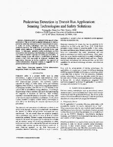
classification. Figure 1 shows an overview of our method.
1 m+n
Enter the adaboost iteration, set the iteration times as T 1). Normalize the sample weight as follows:
ω ωi∗,t = m + n i ,t ∑ ωi,t
(5)
i =1
ωi∗,t represents the normalized weight ωt ,i sample i in iteration t .
Where
of
2).All the weak classifiers are tested on the training sample set. For each classifier, collect all the misclassified samples, and sum up their weights to obtain classification error ε j , where j indicates the index of the weak classifiers. Choose the one with the least error. 3).Use the chosen classifier to perform classification on all samples. If the sample is correctly classified, maintain its weight, otherwise, change it according to the equation below.
ωt∗+1,i = ωt∗,i βt1−e
(6)
i
Where ei equals the classification result; when correctly
βt = 4.
detected,
εt ; εt 1− εt
ei =0, otherwise ei =1;
stands for the minimum error related
to the chosen weak classifier. After all T iterations, the final strong classifier obtained from cell k is as follows: Ν
N
1 ⎧1 if ⎪ ∑ α t hk ,t ( X i ) > ∑ α t Hk (Xi ) = ⎨ 2 t =1 t =1 ⎪⎩0 otherwise 1 Where α t = log βt
(7)
As the output H k ( X i ) of the adaboost is a strong classifier, Ν
the weighted sum of weak classifiers
∑α h t =1
t k ,t
( X i ) in cell
k must contain important information that differentiates pedestrians from other objects. This forms the new feature in our approach, which we name as boosted HOG feature. The feature vector is built by combining them from all cells. A linear SVM is used to train on the feature vector for the final 1157
Fig.1. An overview of our approach. Note that three types of basic HOG features are used. The idea of using blocks of various sizes is intended to capture both local and global shape information in pedestrian objects.
II. EXPERIMENTS AND PERFORMANCE STUDY A. Datasets and Methodology The INRIA pedestrian dataset (available at: http://pascal.inrialpes.fr/data/human/ ) is used in the training and testing phase of our algorithm. The dataset contains 2416 positive training samples in the folder ‘96X160H96’ with resolution at 160x96 and 1126 positive testing samples in ’70X134X96’ with resolution at 134x70. For negative training samples, a total of 12180 128x64 patches are sampled randomly from 1218 negative images in the folder ‘\train\neg’. To obtain the negative testing set, we sample 10 patches from each negative image in folder ‘\test\neg’ to obtain 4530 negative samples. For simplicity we only use cropped samples rather than whole images to test our approach. Our algorithm implements 3 groups of boosted HOG features. The conventional 16x16 block could achieve a dense scan on the image and capture local features that differentiate pedestrians from other objects. However, only local information is inadequate to extract global shape features like the body contour. To address this problem, we use 3 types of blocks: 1).Boosted HOG #1 with block size=16x16, cell size=8x8, block stride=8 and 105 blocks over the 128x64 region. 2).Boosted HOG #2 with block size=32x32, cell size=16x16, block stride=8 and a total of 65 blocks over 128x64 region. As in most samples the head and shoulder region of pedestrians span an area about 32x32, we expect
the 32x32 block could help capture more information in the head and shoulder region. 3).Boosted HOG #3 with block size=64x32, cell size=32x16, block stride=16.This gives an extra 15 blocks, and due to the block’s larger size, it covers most of the body trunk and helps obtain more global information. It is worth noting that although computing HOG of variably-sized blocks also appear in [9], our approach apparently differs from the one proposed by Zhu et al. In [9], the authors construct a rejection cascade. In each level they build a strong classifier with adaboost. The weak classifiers they use are linear SVM using a 36D HOG of each block. In contrast, the weak classifier in our algorithm is derived from the bin value of HOG in a cell; moreover, we use adaboost only to create a novel feature that has 4 dimensions within each block. There is no classifier cascade and when 3 groups of boosted HOG are ready, we only perform classification once to obtain the final output. Our approach is coded in Matlab and during the SVM training and testing phase, the SVM-lite 6.01/ MATLAB MEX Interface [15] is implemented. Our approach to detection contains the following steps: 1). Train boosted HOG #1 with 2416 positive and 2436 negative samples. 2).With the obtained feature, train SVM with 2416 positive samples and 12180 negative samples. Test the obtained SVM on the same training set. Record all the false positive and false negative samples. 3). Use the above false positive samples and false negative samples in step 2 to train boosted HOG #2. 4). Train boosted HOG #3 with the same training set in step 1. 5). Combine boosted HOG #1, #2, #3 feature to form the feature vector and train the linear SVM classifier. 6). Classify test samples with the obtained SVM. B. Parameter settings In our approach several parameters are crucial in maintaining the performance of our detector. 1) The number of negative samples negsize in the training of the first boosted HOG: during our adaboost training, we choose several configuration of negsize to examine its influence on the performance of the detector. Figure (2) shows the classification performance with 2416 positive samples where negsize=1218(one negative patch per image), 2436(two negative patches per image), 4872(four negative patches per image) and 6090(five negative patches per image).As the figure shows, when the number of negative training sample negsize deviates too much from that of the positive sample the performance of our detector decreases sharply. Therefore we use 2436 negative samples as the optimum parameter to train the boosted HOG#1. 2).The binnumber in the HOG feature: in Dalal’s paper [1], they uniformly select 9 orientations in the range 0 to 180 degrees. In our experiment we examine the algorithm performance with binnumber equal to 8, 9, 10, and 15. As
Fig.2. effect of different values of negsize
Figure (3) shows, when 8 directions are chosen within 0 to 180 degrees, the detector can only achieve moderate performance however as the binnumber grows the accuracy of our detector improves. However the performance would decrease when binnumber values are beyond 10. Therefore our experiment suggests that binnumber=10 should be the optimum value for classification.
Fig.3. effect of binnumber
3). The Adaboost iteration T: we test the performance of our detector with T=5, 10, 15, 20. The resulting DET curve in figure (4) shows that an iteration of 5 is inadequate to take advantage of adaboost to improve the discriminative power. The performance is improved when more iterations are involved. To achieve satisfactory result the iteration T should at least be 10. 4). When training the final SVM classifier, the negative sample size N could affect the quality of the classifier; therefore we compare the performance curve of different sizes of negative samples. We choose N=2436(two negative patches per image), 5000(first 500 non-pedestrian images in all 1218 negative ones), 6090(five negative patches per image) and 12180(ten negative patches per image) for comparison. As Figure (5) demonstrates, our detector achieves best result when N=6090 (five patches per negative image), which implies that more negative training sample could result in better detection; however the fact that when N is set to 12180, the detector performance deteriorates has reduced this
1158
Fig.4. effect of iteration T
Fig.6. effect of different training strategies
possibility. This is perhaps due to one of the disadvantages of adaboost e.g. sensitivity to noise.
We tried several groups of test data and two of them are shown in figure (7). As it shows, our detector achieves comparable performance like HOG. Due to the limitation on the number of testing negative samples in our experiment, we can not observe the miss rate of both algorithms with FPPW=1e-4; we notice when FPPW is lower than 1e-3 the miss rate of our approach is almost the same as that of HOG.
Fig.5. effect of negative sample size N
C. Performance Study In our experiment we compare the performance of our detector under different training strategies. As figure (6) illustrates, we tried two approaches in training boosted HOG#2. One is with full training set of 2416 positive and 2436 negative samples and the other is with the false positive and false negative sample sets obtained from step 2 in our 6-step detection approach. The curve in figure (6) clearly shows that in this way the obtained feature can better differentiate between pedestrians and other similar objects. Moreover, the DET curves prove that the inclusion of boosted HOG #3 produces a promising effect on the final detector. With the information from 64x32 blocks the miss rate of the detector is further decreased. We compare the performance of our detector with that of the Dalal’s detector implementing HOG feature. We test the HOG detector with the binary code [17] published online, and choose the following parameter in running our algorithm: negsize=2436, binnumber=10, T=15, N=6090(five negative patches per image). We experiment on the INRIA test dataset, which includes 1126 positive and 4530 negative samples. The DET curves are illustrated in figure (7).
Fig.7. comparison between HOG and boosted HOG
Though our detector performs quite well with many hard samples correctly classified, it still fails to correctly detect some samples. As figure (8) shows, irregular postures like riding bicycles and bad illumination result in several false negative samples. And as in boosted HOG feature we use the combination of bin values of HOG rather than bin values themselves, the information in cells indicating the distribution of strong or weak gradients in certain directions and positions is not fully used. As a result, some negative samples having similar boosted HOG values though not geometrically mimicking pedestrian’s contour, are falsely classified. Besides performing equally well like the HOG, the boosted HOG leads to a much smaller feature vector. The total size of our feature vector includes three parts, i.e. boosted HOG #1, #2, and #3.The total feature has 420+260+60=740 dimensions compared with 105*4*9=3780 in HOG. Our detector achieves the same results with the size of the feature
1159
of negative sample in SVM training could greatly influence the classification accuracy; the underlying reason for this should be further studied. Moreover the evaluation of computation cost should involve more statistic information. In our experiment, steps such as the ROI selection and the fusion of classification results are not included. These issues form the focus of our future work.
(a)
REFERENCES [1] [2] (b) Fig.8. some (a) false negative and (b) false positive samples in our test.
[3]
only 19.6% of the HOG. This results in considerable reduction of storage requirement in both training and testing phase. When feature vector has smaller size, the computation cost in SVM testing could also be reduced. As Gordan et al. [16] demonstrate, the decision function of a linear SVM has the following form: NS
f ( x) = ∑ α q yq xT xq
[5] [6]
(8)
q =1
N S represents the total number of support vectors in the trained classifier; xq is equal to qth support vector; Where
αq
[4]
[7] [8]
is the Lagrange multiplier for support vector xq ; yq is the
category of
xq ; and x is the feature vector of a testing
sample. The equation (8) demonstrates that when classifying an unknown sample, the computation cost of the linear SVM is related to H, the size of the feature vector x and the size of the support vector
N S .The dot product x xq contains 2*H
vectors in both the training of HOG and of our detector. The ratio of elementary operation in SVM computation is:
Chog
=
[10]
T
elementary operations. So the total number of elementary operation is 2* N S *H. We record the number of support
Cboosted hog
[9]
557 * 2*740 = 7.97% 1368* 2*3780
(9)
[11] [12] [13] [14]
The equation (9) shows that in the experiment our algorithm could greatly reduce the computation cost.
[15]
III. CONCLUSION In this paper we propose a novel feature for pedestrian detection in static images. The basic HOG feature is adopted and trained with adaboost to obtain the boosted HOG feature. A linear SVM is trained to perform the detection. The experiment shows that our approach achieves comparable results as the HOG detector with much smaller computation cost and storage requirement.However several important parameters are tested to examine their effects on the performance of the algorithm. The results show the size of negative samples in training boosted HOG#1 and the number
[16]
[17]
1160
N. Dalal and B. Triggs. “Histograms of oriented gradients for human detection”. Int. Conf. on Computer Vision and Pattern Recognition, volume 2, pages 886–893, June 2005. C. Papageorgiou and T. Poggio. “A trainable system for object detection”. IJCV, 38(1):15-33, 2000. L. Zhao and C. Thorpe, “Stereo and neural network-based pedestrian detection,” IEEE Trans. Intelligent Transportation. System, vol. 1, no. 3, pp. 148–154, Sep. 2000. P. Viola, M. J. Jones, and D. Snow. “Detecting pedestrians using patterns of motion and appearance”. The 9th ICCV, Nice, France, volume 1, pages 734-741, 2003. B. Leibe, E. Seemann, and B. Schiele, “Pedestrian detection in crowed scenes,” in Proc. IEEE Conf. on Computer Vision and Pattern Recognition, vol. 1, pp. 878–885, Jun. 2005 K. Mikolajczyk, C. Schmid, and A. Zisserman. “Human detection based on a probabilistic assembly of robust part detectors”. The 8th ECCV, Prague, Czech Republic, volume I, pp. 69-81, 2004. I. P. Alonso et al. "Combination of feature extraction methods for SVM pedestrian detection." IEEE Trans. Intelligent Transportation Systems, 8(2): 292-307, 2007. M. Bertozzi, A. Broggi, M. Del Rose, M. Felisa, A. Rakotomamonjy and F. Suard. “A pedestrian detector using histograms of oriented gradients and a support vector machine classifier”. Intelligent Transportation Systems Conference, 2007. Q. Zhu, S. Avidan, M.C. Yeh, and K.T. Cheng. “Fast human detection using a cascade of histograms of oriented gradients”, IEEE Computer Society Conference on Computer Vision and Pattern Recognition, 2006. P. Sabzmeydani and G. Mori. “Detecting pedestrians by learning shapelet features”. IEEE Conf. on Computer Vision and Pattern Recognition, 2007. A. Mohan, C. Papageorgiou, and T. Poggio. “Example-based object detection in images by components”. PAMI, 23(4):349-361, April 2001. Y. Ke and R. Sukthankar. “PCA-SIFT: A more distinctive representation for local image descriptors”. CVPR, Washington, DC, USA, pages 66-75, 2004. S. Belongie, J. Malik, and J. Puzicha. “Matching shapes”. The 8th ICCV, Vancouver, Canada, pages 454-461, 2001. D. G. Lowe. “Distinctive image features from scale-invariant keypoints”. IJCV, 60(2):91-110, 2004. The software is an extension developed by Tom Briggs to the Joachims’s SVM-lite package. T. Joachims, “Making large-scale SVM learning practical”. Pages: 169 – 184. In B. Schlokopf and C. Burges and A. Smola (ed.) “Advances in kernel methods - support vector learning”,MIT-Press,1999.Available:http://webspace.ship.edu/thbrig/ mexsvm/svm_mex601.tar.gz M. Gordan, A. Georgakis, O. Tsatos, G. Oltean, L. Miclea. "Computational complexity reduction of the support vector machine classifiers for image analysis tasks through the use of the discrete cosine transform," IEEE Int. Conf. on Automation, Quality and Testing, Robotics , vol.2, no., pp.350-355, May 2006 Available: http://pascal.inrialpes.fr/soft/olt/OLTbinaries.zip