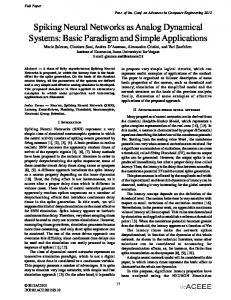
Focus here on auditory perception, auditory Scene Analysis and Spiking. Neurones .... or CSM), the spiking neural network generates the mask (binary gain) to.
Perceptive, non-linear speech processing and spiking Neural Networks Jean ROUAT, Ramin PICHEVAR and St´ephane LOISELLE http://www.gel.usherb.ca/rouat/ UNIVERSITE´ DE SHERBROOKE D´epartement de g´enie e´ lectrique et de g´enie informatique Laboratoire de Traitement de Signal et de Neurosciences computationnelles Int. Summer School on Neural Nets ’E.R. Caianiello’, 9th. Course Vietri sul Mare - Italy, 13-18 Sept. 2004
14 September 2004 •First •Prev •Next •Last •Go Back •Full Screen •Close •Quit
Sommaire 1
Corrupted Speech Processing
3
2
The auditory system
4
3
Basic notion of spiking neurone models
12
4
Real neurones: that clean?
16
5
Auditory Scene Analysis
17
6
Example : Sources separation with a multi-representation and temporal correlation 20
7
Dynamic Link Matching - Temporal Correlation
32
8
Exploration in speech recognition
35
9
General Conclusion
43
10 Intuitive notions of Pattern Recognition via Spiking Neurones
44
•First •Prev •Next •Last •Go Back •Full Screen •Close •Quit
1. Corrupted Speech Processing • Conception of algorithms and systems for audio processing based on conventional approach and auditory system knowledge
• Focus here on auditory perception, auditory Scene Analysis and Spiking Neurones http://www-edu.gel.usherb.ca/pichevar/Demos.htm /di//da/ separated /da/ separated /di/ one microphone Separation made with Spiking N.N. [1] Speech plus other sources (siren) Separation made with Spiking N.N. [1] speech and siren separated siren separated speech one microphone Speech plus noise (relatively stationary source: music) Mask by adapted wavelet thresholding [2] [3] before processing after processing one microphone http://Jean-Marc Valin, Ph.D. student, Or this site (if the first does not work): http://Jean-Marc Valin, Ph.D. student Speech plus interfering speech (3 speakers) 8 microphones Separation made by beamforming and postprocessing [4] •First •Prev •Next •Last •Go Back •Full Screen •Close •Quit
2. The auditory system Peripheral ear, physiology From the site http://www.cochlea.info by [5] • External ear [5] External ear for acoustic beamforming (directional antenna and resonator). • Middle ear [5] Middle ear as an impedance adapter. • Inner ear [5] Inner ear: the vestibule as the organ of equilibrium and the cochlea for hearing. • Cochlea [5] Cochlea : the sophisticated organ. • The organ of Corti [5] The organ of Corti: the coder. • OHC active and IHC passive processes [5] The coder in action. • Innervation [5] Innervation of the cillia cells. •First •Prev •Next •Last •Go Back •Full Screen •Close •Quit
Electrical responses of hair cells and fibers: I From the site http://www.cochlea.info by [5] • hair cell responses [5] Lower frequency fibres can synchronise on characteristic frequency of the fibre. High frequency fibres synchronise mostly on the envelope. • Middle ear [5] brainstem evoked auditory potentials (BAEPs)
•First •Prev •Next •Last •Go Back •Full Screen •Close •Quit
Electrical responses of hair cells and fibers: II Because of Copyrights, it is not possible to include the figure, please contact me (J.Rouat) or refer to the book: C. K. Henkel. The Auditory System. In Duane E. Haines, editor, Fondamental Neuroscience. Churchill Livingstone, 1997. Response characteristics of type I afferent fibres. (A), Frequency tuning curves; (B), Post-stimulus time histogram of discharges trough the duration of a tone burst at the characteristic frequency of a primary afferent fibre; (C), Discharge rate in function of sound pressure at the characteristic frequency of the fibre. From [6]
•First •Prev •Next •Last •Go Back •Full Screen •Close •Quit
Responses of Cochlear Nucleus neurones Because of Copyrights, it is not possible to include the figure, please contact me (J.Rouat) or refer to the book: C. K. Henkel. The Auditory System. In Duane E. Haines, editor, Fondamental Neuroscience. Churchill Livingstone, 1997. Cell types in the cochlear nucleus, typical responses and major ascending connections. Bushy cells (Primary-like): timing and phase − > binaural hearing, multipolar cells (Chopper): changes in sound pressure level (AM) − > direct monoaural pathway, octopus cells (Onset) with broad frequency tuning − > monoaural indirect pathway. From [6]
•First •Prev •Next •Last •Go Back •Full Screen •Close •Quit
Cochlear Nuclei Because of Copyrights, it is not possible to include the figure, please contact me (J.Rouat) or refer to the book: C. K. Henkel. The Auditory System. In Duane E. Haines, editor, Fondamental Neuroscience. Churchill Livingstone, 1997. (A) and (C): Dorsal and ventral cochlear nuclei in cross section; (B): The ventral cochlear nucleus extends rostral to the dorsal nucleus. From [6]
•First •Prev •Next •Last •Go Back •Full Screen •Close •Quit
Auditory system signal processing Neural Responses from the Auditory Cortex of a rat
Two tonalities with variable intensity (auditory cortex, ewaked rat). (laboratoire de Neuro-heuristique, Institut de Physiologie, Universit´e de Lausanne, Suisse, May 1996).
•First •Prev •Next •Last •Go Back •Full Screen •Close •Quit
General observations • Oscillatory noisy response of neurones; • Neurone with higher sensitivity − > longer response; • Pattern recognition: find the cells that fire coherently; • Enhancement of transients at the cortical level; • Similar stimulus − > same timing of the spikes; • Specific receptive field of neurones − > specialised neurones; • Geographical localisation yields recognition.
•First •Prev •Next •Last •Go Back •Full Screen •Close •Quit
The auditory based approach we presently use 1. Peripheral auditory model (Cochlea and Cochlear Nucleus) [7] [8] [9] [10]. 2. Segmentation of the auditory peripheral representations with networks of oscillatory neurones [11]. 3. Dynamic Link Matching between neurones for source separation or for recognition [12] [1] [13]. 4. Rank Order Coding (ROC) for sequence recognition.
Some common features of our neural networks • The information is coded in the synchronisation of neurones; • There is a topological organisation of the cells; • Synaptic weights are continuously adapted (no training or recognition phase); • The dendritic tree yields analysis and recognition (when combined with thresholding) of sequences of events. • Synchronisation between neurones is detected by thresholding.
•First •Prev •Next •Last •Go Back •Full Screen •Close •Quit
3. Basic notion of spiking neurone models Hodgkin-Huxley model External (sea water)
VNa
VK
VCl
gNa
gK
gCl V(t)
C INa
ICl
IK
IC
I(t) Internal (axoplasm)
Equivalent circuit of a membrane section of a squid axon (from Hodgkin-Huxley, 1952). gCl , gN a and gK are the conductance of the membrane for respective ionic gates. V (t) is the membrane potential when I(t) = 0 (no external input). •First •Prev •Next •Last •Go Back •Full Screen •Close •Quit
Leaky Integrate and Fire models I(t) C
R
V(t)
Equivalent circuit of a leaky integrate and fire neurone (LIF). C: membrane capacitance, R: membrane resistance, V: membrane potential.
I(t) is the sum of the current going trough the capacitance plus the resistance current. The subthreshold potential V (t) is given by: dV (t) V (t) + (1) dt R(t) V (t) is the output, I(t) is the input. When V (t) crosses a predetermined threshold δ(t), the neuron fires and emits a spike. Then V (t) = Vr , where Vr is the I(t) = C(t)
resting potential.
•First •Prev •Next •Last •Go Back •Full Screen •Close •Quit
Wang and Terman oscillator model It is a modified version of the Van der Pol relaxation oscillator (Wang-Terman oscillators [14]).
dx = 3x − x3 + 2 − y + ρ + I + S dt
(2)
dy = �[γ(1 + tanh(x/β)) − y] dt
(3)
• x is the membrane potential (output) of the neurone and y is the state for channel activation or inactivation. • ρ denotes the amplitude of a Gaussian noise, I is the external input to the neurone. • S is the coupling from other neurones (connections through synaptic weights). • �, γ , and β are constants.
•First •Prev •Next •Last •Go Back •Full Screen •Close •Quit
The spiking neural models we use for source separation
Example of neuron’s output for the W-T oscillator. Implementation by relaxation oscillators, chaotic neurones or leaky integrate and fire neurones have been tested [15]. •First •Prev •Next •Last •Go Back •Full Screen •Close •Quit
4. Real neurones: that clean?
Enhancement comparisons of extracellular potentials (collaborative work with CHU Grenoble).
Signal Enhancement prior to spikes sorting of extracellular potentials (collaborative work with CHU Grenoble). •First •Prev •Next •Last •Go Back •Full Screen •Close •Quit
5. Auditory Scene Analysis • Find a suitable signal representation (auditory image representation)
(a) Spectrogram of a /di/ and /da/ mixture. (b) Spectrogram of /di/ plus siren mixture.
• Analyse the auditory scene and segment objects. • Segregate objects belonging to the same source (use a mask). •First •Prev •Next •Last •Go Back •Full Screen •Close •Quit
Auditory Scene Analysis (Bregman) [16] From : http://dactyl.som.ohio-state.edu/Huron/Publications/huron.Bregman.review.html • Analogies with the the visual system. • Most sounds have a history. The mental images of lines of sound are auditory streams. Study of the behavior of such images is: auditory streaming.
•First •Prev •Next •Last •Go Back •Full Screen •Close •Quit
Auditory Scene Analysis (ctd) • Auditory streaming is fundamental to the recognition of auditory events since it depends upon the proper assignment of auditory properties to different sound sources. • How sounds cohere to form a sense of continuation is the subject of stream fusion. Since more than one source can sound concurrently, a second domain of study is how concurrent activities retain their independent identities – the subject of stream segregation . Stream-determining factors include: timbre (spectral shape), fundamental frequency (pitch) proximity, temporal proximity, harmonicity, intensity, and spatial origin. In addition, when sounds evolve with respect to time, it is possible for them to share similarities by virtue of evolving in the same way. In Gestalt psychology, this perceptual co-evolution of parts is known as the principle of common fate . Bregman has pointed out that the formation of an auditory stream is governed largely by this principle.
•First •Prev •Next •Last •Go Back •Full Screen •Close •Quit
6. Example : Sources separation with a multirepresentation and temporal correlation CSM Generation
Envelope Detection
CAM Generation
Neural Synchrony
Spiking Neural Network
Mask Generation
256
256 256
Synthesis Filterbank
256
256
Analysis Filterbank
Sound Mixture
Separated Signals
Source Separation System. Depending on the sources auditory images (CAM or CSM), the spiking neural network generates the mask (binary gain) to switch ON/OFF – in time and across channels – the synthesis filterbank channels before final summation. •First •Prev •Next •Last •Go Back •Full Screen •Close •Quit
Strategy Two representations are simultaneously generated: - Amplitude Modulation map, that we call Cochleotopic/AMtopic (CAM) Map. It somehow reproduces the AM processing performed by multipolar cells (Chopper-S) from the anteroventral (inferior cochlear nucleus [9]. - Cochleotopic/Spectrotopic Map (CSM) that encodes the averaged spectral energies of the cochlear filterbank output. It is closer to the spherical bushy cell processing from the ventral cochlear nucleus [6].
• We assume that different sources are disjoint in the auditory image representation space and that masking (binary gain) of the undesired sources is feasible. Attention will decide which source to keep. • Speech has a specific structure that is different from that of most noises and perturbations [17]. Also, when dealing with simultaneous speakers, separation is possible when preserving the time structure (the probability at a given instant t to observe overlap in pitch and timbre is relatively low). Therefore, a binary gain can be used to suppress the interference (or separate all sources with adaptive masks guided by attentional process). • Temporal correlation is used to find dependencies between channels to simultaneously segregate and bind auditory channels. •First •Prev •Next •Last •Go Back •Full Screen •Close •Quit
Crucial point: the signal representation Example of cochlear filterbank Magnitude Response
FIR implementation of gammatone filters. •First •Prev •Next •Last •Go Back •Full Screen •Close •Quit
GammaChirp filter bank output
(a) No active process from the outer hair cells. (b) Active process is on. Matlab implementation by Toshio Irino [18]. •First •Prev •Next •Last •Go Back •Full Screen •Close •Quit
Auditory maps generation Down–sampling to 8000 samples/s. Filter the sound source using a 256filter Bark-scaled cochlear filterbank ranging from 100 Hz to 3.6 kHz. Our CAM/CSM generation algorithm is as follows: 1. For CAM: Extract the envelope (AM demodulation) for channels 30-256; for other low frequency channels (1–29) use raw outputs (resolved harmonics and hair cells responses). 2. For CSM: Nothing is done. 3. Compute the STFT of the envelopes (CAM) or of the filterbank outputs (CSM) using a Hamming window (Non-overlapping adjacent windows with 4ms or 32ms lengths have been tested). 4. In order to increase the spectro-temporal resolution of the STFT, find the reassigned spectrum of the STFT [19] (this consists of applying an affine transform to the points in order to realocate the spectrum). 5. Compute the logarithm of the magnitude of the STFT. •First •Prev •Next •Last •Go Back •Full Screen •Close •Quit
Example of CAM parametrisation
Example of a twenty–four channels CAM for a mixture of /di/ and /da/ pronounced by two speakers; mixture at SN R = 0 dB and frame center at t = 166 ms. •First •Prev •Next •Last •Go Back •Full Screen •Close •Quit
Example of CSM parametrisation
CSM of the mixture of /di/ and a siren at (a) t=50 ms (b) t=200 ms.
•First •Prev •Next •Last •Go Back •Full Screen •Close •Quit
Network architecture
Neural Architecture Global Controller
Fully Connected Network
Partially Connected Network
Univ. de Sherbrooke
Jean Rouat, NOLISP03, 20 May 2003, Le Croisic
Architecture of the Two-Layer Bio-inspired Neural Network. G: Stands for global controller (the global controller for the first layer is not shown on the figure). One long range connection is shown in the figure. •First •Prev •Next •Last •Go Back •Full Screen •Close •Quit
Some equations, . . . First layer: Auditory image segmentation
dx = 3x − x3 + 2 − y + ρ + I + S (4) dt dy = �[γ(1 + tanh(x/β)) − y] (5) dt • x : membrane potential (output) of neurone, y : state for channel activation or inactivation. • ρ : amplitude of a Gaussian noise, I : external input to the neurone, and S is the coupling from other neurones. • �, γ , and β are constants. • A neurone is connected to its four neighbors. The CAM (or the CSM) is applied to the input of the neurones.
•First •Prev •Next •Last •Go Back •Full Screen •Close •Quit
• Weights between neuron(i, j) and neuron(k, m) wi,j,k,m(t) =
1 0.25 Card{N (i, j)} eλ|I(i,j;t)−I(k,m;t)|
(6)
I(i, j), I(k, m) external inputs to neuron(i, j) and neuron(k, m) ∈ N (i, j). • Card{N (i, j)} is equal to 4, 3 or 2 depending on the location of the neuron on the map. • Si,j defined in Eq. 4:
X Si,j (t) =
wi,j,k,m(t)H(x(k, m; t)) − ηG(t) + κLi,j (t)
(7)
k,m∈N (i,j)
• Global controller: G(t) = αH(z − θ) dz = σ − ξz dt
(8) (9)
σ is equal to 1 if the global activity of the network is greater than a predefined ζ and is zero otherwise. α and ξ are constants. • Li,j (t), long range coupling: � 0 j > 30 Li,j (t) = P (10) w (t)H(x(i, k; t)) j ≤ 30 i,j,i,k •First •Prev •Next •Last •Go Back •Full Screen •Close •Quit k=225...256
dz/dt= σ − ξ z G σ=1
σ=0
sum > ζ
sum < ζ −η
Fre q
ue nc
ies
Binding via synchronization
Global Controller
Also network architecture
L i,j Neuron
i,j
Channels
w
Neuron i,j,k,m
H(.)
x(k,m;t)
k,m
CAM/CSM
Architecture of the Two-Layer Bio-inspired Neural Network. G: Stands for global controller (the global controller for the first layer is not shown on the figure). One long range connection is shown in the figure. •First •Prev •Next •Last •Go Back •Full Screen •Close •Quit
Second layer: temporal correlation and multiplicative synapses
• Each 256 neurone represents a cochlear channel of the analysis/synthesis filterbank. • For each presented auditory map, binding is established between neurones which entry is dominated by the same source. • Dendrites establish multiplicative synapses with first layer. • neurones belonging to the same source synchronise (same spiking phase) • neurones belonging to the other source desynchronise (different spiking phase). •First •Prev •Next •Last •Go Back •Full Screen •Close •Quit
7. Dynamic Link Matching - Temporal Correlation Segregation and fusion are performed in one step
Illustration of temporal correlation •First •Prev •Next •Last •Go Back •Full Screen •Close •Quit
Criteria example for separation Two criteria to separate the sources:
• Weight values between neurones from 2nd layer (higher correlation between channels yields greater synaptic weights);
• Firing time (neurones whith the same firing instant phase characterise channels dominated by the same source).
Note The Neural Network does not have any apriori knowledge about the nature of the signals.
•First •Prev •Next •Last •Go Back •Full Screen •Close •Quit
Example: separation of speech from telephone trill
Frequency (Hz)
4000
0 0
1.51 Time (s)
Mixture of the utterance ”Why were you all weary?” with a trill telephone noise.
Frequency (Hz)
4000
Frequency (Hz)
4000
0 0
1.51 Time (s)
0 0
1.51 Time (s)
Left: The synthesised ”Why were you all weary?” after separation. Right: The synthesised trill phone after separation. •First •Prev •Next •Last •Go Back •Full Screen •Close •Quit
8. Exploration in speech recognition • Oded Ghitza proposed in 1994 and 1995 the use of auditory periphery model for speech recognition [20, ?] that takes into account the variability of neurone’s internal threshold. • He introduces the notion of Ensemble Interval Histograms (EIH). That representation preserves the spike time intervals information coming from a population of primary fibres. • Speech recognition experiments are made on the TIMIT database by using a mixture of Gaussian Hidden Markov Models. He observes that the EIH representation is more robust on distorded speech when compared to MFCC. • He might have obtained better results by preserving the order of the neurone’s discharges? • In a collaborative work, we explore here the feasability of using the Rank Order Coding as introduced par S. Thorpe and his team [21, 22].
•First •Prev •Next •Last •Go Back •Full Screen •Close •Quit
Definition of the EIH
Cochlear filterbank outputs are compared to thresholds to generate spikes; figure from [20]. •First •Prev •Next •Last •Go Back •Full Screen •Close •Quit
Rank Order coding
Order-of-Arrival neurons
@1
Let the input lines @1,.@4 have increasing weights. If, as in a), stimulation on these lines arrives in this same order then the activation might increase with each arrival and a pulse generated after the last arrival.
@2 @3 @4
Weight modification factor
If, as in b), the order of arrival does not agree with that of the weights, activation may not build up sufficiently to cross the threshold and fire This is because the weights are uniformly decreased with each input arrival as in c).
c) Input arrival order @1
@2
@3
input
@4
@4
@3
@2
@1
input
threshold activation
activation
output
output
a)
b)
Neurone N fires on a specific sequence (A,B,C,D,E). Other sequences will not sufficiently excite N (inhibition variable neurone I) ([23, 24]. •First •Prev •Next •Last •Go Back •Full Screen •Close •Quit
Analysis system
Spikes are generated when the signal amplitude exceeds a threshold. These thresholds act crudely as neurones possessing different excitation levels. •First •Prev •Next •Last •Go Back •Full Screen •Close •Quit
Training
Example of analysis output for digit ’four’.
Example of weights values for digit ’four’. •First •Prev •Next •Last •Go Back •Full Screen •Close •Quit
Reference System: HMM A Hidden Markov Model based system has been trained on the same training set. The system uses hidden Markov models and twelve cepstral coefficients for each time frame [25, 26].
Each word is modeled by a Gaussian Hidden Markov Model with five states.
•First •Prev •Next •Last •Go Back •Full Screen •Close •Quit
Preliminary results French digits spoken by five men and four women. Each speaker pronounced ten times the same digit. Various training strategies have been tested (from 9 pronunciations per digit in the training set to only 1 pronunciation per digit). Recognition has been performed on the 10 pronunciations.
With the biggest training sets, HMM outperforms our ROC prototype, but with the smallest training sets, HMM is not able to converge during training yielding recognition rates as low as 50% while the prototype seats around 65%. •First •Prev •Next •Last •Go Back •Full Screen •Close •Quit
Summary • Even if the system is very crude, interesting performance are obtained with a very limited training set. With only one neurone connected to each cochlear channel, the system yields 65% recognition rate (with one pronunciation per digit). • For each neurone, our prototype uses only the first firing instant of that neurone (emphasis is then generally made on first milliseconds of the signal) while the HMM recogniser uses the full signal. • Careful interpretation should be made. • We were expecting worst results.
•First •Prev •Next •Last •Go Back •Full Screen •Close •Quit
9. General Conclusion • I want an intelligent, robust and autonomous speech recognition system. • Integration of psychology, of psychoacoustics, of neurophysiology, of computer science, of signal processing, of phonetics, etc. is a must if we want to solve the speech recognition problem on long-term and on solid basis. • In this talk, I illustrated two potential partial solutions to the problem of speech recognition. a
Acknowledgements This work has been funded by NSERC, MRST of Qu´ebec gvt., Universit´e de Sherbrooke and by Universit´e du Qu´ebec a` Chicoutimi. Many thanks to our COST277 collaborators : Christian Feldbauer and Gernot Kubin from Graz University of Technology for fruitful discussions on analysis/synthesis filterbanks, Simon Thorpe and Daniel Pressnitzer for discussions on ROC and for receiving S. Loiselle during his 2003 summer session in CERCO, Toulouse. a
Copies of the paper have been distributed yesterday. Please, do no hesitate to give me scientific and ENGLISH feedback. •First •Prev •Next •Last •Go Back •Full Screen •Close •Quit
10.
Intuitive notions of Pattern Recognition via Spiking Neurones
Examples of objects recognition Oscillatory Dynamic Link Matching for Pattern Recognition, R. Pichevar & J. Rouat [13] 1. Image Segmentation 2. Dynamic Link Matching between 2 layers of spiking neurones
Network architecture •First •Prev •Next •Last •Go Back •Full Screen •Close •Quit
Network activity when a bar is presented to the 2 layers Horizontal bar presented to the first layer Vertical bar presented to the second layer No training, no supervision to be required
Activity of first and second layers of the neural map. Colors represent relative phase of oscillations.
•First •Prev •Next •Last •Go Back •Full Screen •Close •Quit
Activity of 6 neurones in one layer Neurones belonging to the same object jointly fire The firing phase, in this context, is the recognition criteria It is very robust to noise and interference
3 neurones in the red, 3 neurones in the blue
•First •Prev •Next •Last •Go Back •Full Screen •Close •Quit
References [1] R. Pichevar and J. Rouat. Cochleotopic/AMtopic (CAM) and Cochleotopic/Spectrotopic (CSM) MAP based sound source separation using relaxation oscillatory neurons. In IEEE Workshop on Neural Networks for Signal Processing, pages 657– 666, September 15-17 2003. [2] M. Bahoura and J. Rouat. Wavelet speech enhancement based on the Teager Energy Operator. IEEE Signal Processing Letters, 8(1):10–12, Jan 2001. [3] M. Bahoura and J. Rouat. A new approach for wavelet speech enhancement. In proceedings of Eurospeech 2001, September 2001. Paper nb: 1937. [4] Jean-Marc Valin, Franc¸ois Michaud, Jean Rouat, and Dominic L´etourneau. Robust sound source localization using a microphone array on a mobile robot. In IEEE/RSJ-Int. Conf. on Intelligent Robots & Systems, Oct. 2003. [5] R. Pujol et al. Cric, montpellier : Audition promenade round cochlea. www.iurc.montp.inserm.fr/cric/audition/english. [6] C. K. Henkel. The Auditory System. In Duane E. Haines, editor, Fondamental Neuroscience. Churchill Livingstone, 1997. [7] Jean Rouat. Nonlinear operators for speech analysis. In M. Cooke, S. Beet, and M. Crawford, editors, Visual representations of speech signals, pages 335–340. J. Wiley and Sons, 1993. [8] Jean Rouat. A nonlinear speech analysis based on modulation information. In A. Rubio and J. Soler, editors, Speech Recognition and Coding, New Advances and Trends, pages 341–344. Springer-Verlag, 1995. [9] Ping Tang and Jean Rouat. Modeling neurons in the anteroventral cochlear nucleus for amplitude modulation (AM) processing: Application to speech sound. In Proc. Int. Conf. on Spok. Lang. Proc., page Th.P.2S2.2, Oct 1996. [10] Ping Tang, Pierre Dutoit, Alessandro Villa, and Jean Rouat. Effect of the membrane time constant in a model of a chopperS neuron of the anteroventral cochlear nucleus : a neuroheuristic approach. In Assoc. for Res. in Oto., 20th. res. meeting, pages P–472, feb 1997. http://www.aro.org/archives/1997/472.html. [11] J. Rouat and R. Pichevar. Nonlinear speech processing with oscillatory neural networks for speaker segregation. In proceedings of EUSIPCO 2002, Sept. 2002. invited.
•First •Prev •Next •Last •Go Back •Full Screen •Close •Quit
[12] R. Pichevar and J. Rouat. Double-vowel segregation through temporal correlation: A bio-inspired neural network paradigm. In NOLISP03, Non Linear Speech Processing, 20–23 May 2003. [13] R. Pichevar and J. Rouat. Oscillatory dynamic link matching for pattern recognition. In 5th neural coding workshop, September 2003. [14] D. Wang and G. J. Brown. Separation of speech from interfering sounds based on oscillatory correlation. IEEE Transactions on Neural Networks, 10(3):684–697, May 1999. [15] R. Pichevar, J. Rouat, C. Feldbauer, and G. Kubin. A bio-inspired sound source separation technique in combination with an enhanced FIR gammatone Analysis/Synthesis filterbank. In EUSIPCO Vienna, 2004. [16] Al Bregman. Auditory Scene Analysis. MIT Press, 1994. [17] J. Rouat. Spatio-temporal pattern recognition with neural networks: Application to speech. In Artificial Neural NetworksICANN’97, Lect. Notes in Comp. Sc. 1327, pages 43–48. Springer, 10 1997. Invited session. [18] Roy D. Patterson, Masashi Unoki, and Toshio Irino. Extending the domain of center frequencies for the compressive gammachirp auditory filter. JASA, 114(3):184–192, September 2003. [19] F. Plante, G. Meyer, and W. Ainsworth. Improvement of speech spectrogram accuracy by the method of reassignment. IEEE Trans. on Speech and Audio Processing, pages 282–287, 1998. [20] Oded Ghitza. Auditory models and human performance in tasks related to speech coding and speech recognition. IEEE TrSAP, 2(1):115–132, 1 1994. [21] S. Thorpe, D. Fize, and C. Marlot. Speed of processing in the human visual system. Nature, 381(6582):520–522, 1996. [22] S. Thorpe, A. Delorme, and R. Van Rullen. Spike-based strategies for rapid processing. Neural Networks, 14(6-7):715– 725, 2001. [23] Rufin VanRullen and Simon J. Thorpe. Surfing a spike wave down the ventral stream. Vision Research, 42(23):2593–2615, august 2002. [24] Bernard P. Zeigler. Discrete event abstraction: An emerging paradigm for modeling complex adaptative systems. Adaptation and Evolution, Oxford Press, 2003. •First •Prev •Next •Last •Go Back •Full Screen •Close •Quit
[25] St´ephane Loiselle. Syst`eme de reconnaissance de la parole pour la commande vocale des e´ quations math´ematiques. Technical report, Universit´e du Qu´ebec a` Chicoutimi, august 2001. [26] St´ephane Loiselle. Exploration de r´eseaux de neurones a` d´echarges dans un contexte de reconnaissance de parole. Master’s thesis, Universit´e du Qu´ebec a` Chicoutimi, 2004.
•First •Prev •Next •Last •Go Back •Full Screen •Close •Quit