Perceptual Grouping of Edges and Corners: Grammatical Inference for Implicit Object Reconstruction from 2-Manifold 3D-Data Peter Michael Goebel∗
Markus Vincze†
Abstract The work of this paper shows how perceptual grouping can be applied within a recently presented framework to support learning of object reconstruction recipes by grammatical inference. Furthermore, the ability to collect information of views from different viewpoints enables us to deal with implicit object topology. We use the perceptual grouping of depth image points into planes by probabilistic robust fitting and the segmentation of edges and corners by intersecting the planes. The edge and corner primitives found by processing of Monte-Carlo simulations and real depth images, are used to train a N-gram model that build object prototypes by Bayesian belief networks. We use perplexity to find out the best performing belief network under candidates. The modeling approach can be utilized for the representation and recognition of object types with occlusions in cluttered, and noisy environments.
1
Introduction
Psychological findings of mammalian visual perception generate supports for cognitive vision models in machine-vision in that they assume the most regular and simplest organization that is equivalent with an image of a given setup [21]. Hence, Gestalt theory appears to be the root of perceptual grouping (PG) and aims at the detection of structure and regularities over several stimuli by extraction of groups of image features that occurred non-accidental, where the grouping principles are based on similarity, proximity, common fate, collinearity, good continuation and past experience [13]. Thus, a one-to-one mapping is found, which maps geometric primitives to sets of numerical parameters into a subset of Rn , where n is the dimension of the representation [4]. ∗
E-mail:
[email protected] Vision for Robotics Lab., Automation and Control Institute ACIN, Vienna University of Technology. Supported by project S9101 ”Cognitive Vision” of the Austrian Science Foundation. † E-mail:
[email protected] Vision for Robotics Lab., ACIN, Vienna University of Technology.
1
Since identification of objects within a familiar scene is influenced by the observer’s location, reconstruction can be supported by contextual information about where we are in space and in which direction we are looking [3]. Although projective views from objects possess some invariance to viewpoint change [2], they appear very different when the change gets above a certain limit. A general mathematical definition is needed in order to generate appropriate and complete object representations, since it appears rather impossible to collect all necessary information for a reconstruction of object-topology of all possible object-views in advance. In our approach, we find this definition in the notion of manifolds, where the key idea is that all appearing object-views are projections from the same original object and therefore smoothly interrelated. Definition 1.1. When, as shown as in Figure 1 – X is a set of points in Rn , (Ui ⊂ X) an © ª open set, ϕi maps ϕi := Ui ∩ ³ X 7→ Rd ´| d < n of projective representations of the set X ¡ ¢ , ϕj · ϕ−1 are two mappings Rd 7→ Rd infinitely – and Iff {Ui ∩ Uj6=i 6= ∅} and ϕi · ϕ−1 j i differentiable – then the set X together with the open sets Ui and the maps ϕi is called a C ∞ manifold of dimension d (adapted from [4]).
Figure 1: A 2-Manifold: element x ∈ X is represented by a pair (p, i), where p ∈ Rd and i is the index, ϕi such that p = ϕi (x), then the set of pairs (Ui , ϕi ) is called an atlas of set X[4]. However, object reconstruction methods that are state-of-the-art commonly utilize a priori knowledge for each object that should be recognized. To be of practical interest in a real world sense a method must also be able to deal with objects for which it has no explicit prior model ready. In recent work we proposed a cognitive framework [8] with the implementation of an vision module based on mammalian psychophysical findings by using predefined object recipes for object reconstruction [6]. The work of this paper shows how perceptual grouping can be applied within the framework to support learning of object reconstruction recipes by grammatical inference. We use the PG of depth image points into planes by probabilistic robust fitting with RANSAC [5] and the segmentation of edges and corners by intersecting the planes. The edge and corner 2
primitives found by processing of Monte-Carlo simulations and real depth images, are used to train a N-gram model that build object prototypes by Bayesian belief networks. We use perplexity to find out the best performing recipe under candidates. The paper is organized as follow: Section 2 shows related work; Section 3 shows how object detection is related to representation; followed by Section 4 with presenting a N-gram model as the learning corpus; Section 5 concludes with an outlook to future work.
2
Related Work
There exist a vast literature on PG in vision, see e.g. [19] for a survey. Early work in PG dates back to Marr [16], who was first who suggested to incorporate grouping based on curvilinearity into larger structures by his primal sketch approach; Witkin and Tenenbaum [22] postulated non-accidentalness for spatiotemporal coherence; Lowe [15] derived an expectation estimate for accidental occurrences by assuming an uniform distribution to line segments; Sarkar and Boyer [18] developed a Bayesian network method for geometric knowledge-based representation; Zucker [24] introduced closure as more global feature to better deal with occlusions; and Ackermann et al [1] introduced a Markov random field grouping approach with learning from hand-labeled trainings sets; however, this list is still far from completeness. More recent work of Procter [17] investigated grouping of edge-triple features, to recognize polyhedrons from 2D image projections, however, the method turned out to be too sensitive to noise and thus failed practical demonstration. Levinshtein et al [14] proposed recovering a Marr [16] like abstraction hierarchy from a set of examples by applying a multi-scale blob and ridge detector for feature extraction, here draw backs arise from the fact that positional information of the blobs is lost during a graph embedding and that a vast number of parameters are to be defined. Zillich [23] aimed at issues concerning complexity and robustness by proposing an incremental processing scheme for the PG of edges in indoor scenes. He proposed using Gestalt principles to support PG and implemented successfully a Markov random field approach in order to deal with real-world objects. Although, in abstract sense, the approach relates very close to our approach, his self-criticism is, he unfortunately highly assumed the getting of clean edges by local edge detectors, which degraded system performance in complexer setups. The main difference to our approach is that we focus on robustness by applying multiresolution methods [8] and to use more global approaches rather than localized ones. We intend to get first only a coarse representation of an object at hand and refine the representation afterwards when more information is required.
3
3
From Detection to Representations
Objects, seen on a very abstract level, can be represented by graphs. These graphs are representations of the connections between structural elements, such as (i) corners; (ii) edges; and (iii) boundaries, where two areas meet: in a fold1 , or in a blade2 , or a face3 . Structural elements and their connections are defined by relations between image primitives. Image primitives are composed by groupings of image features that are extracted from image points. Thus, the more abstract process is that the structural elements, which constitute an object, are searched in a reduced search space by defining some relations between them. To get ready for corner classification, one has first to segment edges within the image.
3.1
Structural Segmentation in 3D
Image segmentation is commonly the partitioning of an image into regions that separate different areas from each other and also from its background. Because of lack of space, we refer [9] for a comprehensive review of low-level segmentation methods4 . In our present approach we use structural properties such as cutting-edges between intersecting planes that are detected in the 3D-point-cloud of the depth images by using a robust plane grouping method applied in [20]. The method uses the Random Sample Consensus Algorithm (RANSAC) [5], which is a probabilistic algorithm for robust fitting of models in the presence of many data outliers and noise. The plane fitting algorithm randomly selects points from the 3D-point-cloud of the depth image and groups triples together in order to define triangles. Only triples that form triangles that lie within a cube’s face are grouped into planes, where a plane is then defined by its vector to the origin c (center) and its normal vector n that is perpendicular to the plane5 .
3.2
Symbolic Corner Labeling
Depending on the viewpoint, corners may appear very differently. In our approach, we classify corners into four junction types, such as: (L)-type which means an occluding line and denotes a blade that is an object region in front of the background; (Y)-type means a 3-junction, where three surfaces intersect with the angles between each pair are < 180 degree; (T)-type means a 3-junction with one of the angles has exactly 180 degrees; and (W)-type means a 3-junction with one angle > 180 degrees. 1
when both areas are from the same object when one area is from the object and one from the background 3 when one area appears closed 4 Their performance compared to human observers is low, especially when applied in noisy environments. 5 Note the method appears akin to a 3D Hough transform. 2
4
W
Face {XY} n3
p=f .rv3
a3
0
L
RANSAC triangle
c3
c1
Y
gx
W
gy
Junction Classes c2
L
n1 n2
Face {XZ}
z
Face {YZ}
L
x
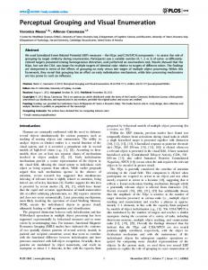
Figure 2: shows the grouping of points from the depth image into planes by RANSAC triangle fitting method. Hence, every face of the cube gets defined its own normal vector n, sitting at the end of the center vector c from the origin O. The intersection of two planes results in a crossing edge g with the space point a. Herein a point p, already on line g, (i.e. p equals the base point f and therefore d = 0) is connected by λ · rv with the endpoint of space point vector a.
4
W
y
gz
Figure 3: a real object’s depth image with the segmentation result, where white marks at the folds represent the final proximity points at the crossing edges. The resulting edge lines are shown in black; the black blade lines are segmented at the border between the depth image face and the object shadow by local segmentation methods. The white crosses depict the location of the corners of the cube, where the 2 faces and the ground plane cross.
Figure 4: the junction-types for corner labeling of an example cube, as used in our approach: (L) means an occluding boarder and denotes a blade where two surfaces meet and just one of them is visible; (Y) means a 3junction, where three surfaces intersect with the angles between each pair are less than 180 degree; and (W) means a 3-junction with one angle greater than 180 degree. Note: no (T)junction type is present here.
The Graphical Model and Grammatical Inference
There exist two principal methodologies in modeling: (i) discriminative, versus (ii) generative approaches. Graphical models are generative approaches, since they may generate synthetic data by sampling from a distribution, define prior probabilities or complete probability distributions. Such models appear commonly too complex for discriminative6 direct estimation of posterior probabilities. Thus, the distributions must be factorized into manageable parts that can be realized by: (i) naive Bayes - assuming strongly naive independence between random variables; (ii) N-grams - which model symbol sequences, using statistical properties; (iii) hidden Markov models - that are Markov processes with unobservable parameters, which 6
e.g. by Support Vector Machines, traditional neural networks, or conditional random fields
5
makes its challenge by determining hidden parameters from the observable ones; and (iv) probabilistic context free grammars - that are context-free grammars, in which each production is augmented with a probability. Hence, a formal grammar is defined by the quadruple G := (N, Σ, P, S); where (N ) is a finite set of nonterminal (syntactical) symbols; (Σ) a finite set of terminal symbols; (P ) a finite set of production rules of the form A → BC, or A → ω, where A, B, C ∈ N and ω ∈ Σ; and (S) the start symbol. A grammar is context-free if (N ∩ Σ) = {} i.e. N, Σ are disjoint sets, and if (∃ string ∈ (N ∪ Σ)∗ : (S, string) ∈ P ); a regular grammar is a finite state automaton which is context-free; regular grammars produce regular languages. Grammatical inference (GI) aims in learning of regular language from examples, i.e. by learning the structure of a finite state automaton and by estimating its transition probabilities [10].
4.1
The Statistical Language N-gram Model
Statistical language models are used for the modeling of sequences of symbols under the assumption that the underlying generation process is an approximate Markov-chain process, where the approximate Markovian property of an order n process is that the conditional probability of future states depends only upon the past n − 1 states, what means that the process is conditionally independent of the > n − 1 past states. Thus, a statistical language model, in general, defines a probability distribution over the set of symbols sampled from a finite alphabet. Its representation by a Markov chain appears as a simple, but high performing concept [11]. The maximal context symbol length is also called the symbols history, where lengths with n = 1 are Uni-gram, n = 2 are Bi-gram, and n = 3 are Tri-gram models. Definition 4.1. A N-gram-Model is a Markov-chain model, giving the probability definition for non-terminating symbols with a maximal context length of n − 1 predecessors by Bayes’ chain rule T Y (1) p(ω) ≈ p(ωt | ωt−n+1 , . . . , ωt−1 ) | {z } t=1
n symbols history
A certain n-tuple of symbols is called a N-gram and is denoted n − G := yz where z is the predicted symbol and y = [y1 , y2 , . . . , yn−1 ] the context length [11]. When one is able to make sure that the training data contain all objects’ data that should be learned, N-gram models have the advantage over hidden Markov language models to allow the calculation of optimum parameters directly from training data. In our present approach, the naive straight ahead solution to the learning problem is to count the absolute frequency c(ω1 , . . . , ωN ) of all symbol tuples and all possible contexts ω1 , . . . , ωN to define all conditional probabilities by relative frequencies. In order to get a satisfying set of sample data, we have tested trigram, bigram and unigram modeling by data from real cube-depth images with different viewpoints and also MC 26
manifold projection simulations of polyhedron objects with 4/4, 8/6, and 20/12 vertices/faces that are tetrahedron, hexahedron, and dodecahedron views, respectively. Figure 5-left, shows a sequence of projections a)...d) of a polyhedron with n = 8 vertices, a cube, where the data was generated by MC simulations; at the middle, the respective planar graphs are given, as described in [6]; and at the right, derived Bayes’ networks are shown that will be discussed in Section 4.2. In Table 1, four unigram transition matrices of MC-samples of Figure 5 are given, showing the observed counts of junction-type to junction-type transitions that are cumulated into training counts for Ni,j | i, j : {L, W, Y, T }, as shown at the left of Table 2. Table 1: Unigram counts of junction to junction dependencies observed from different viewpoints of the Monte-Carlo simulation according to , rows a)...d). Junction to junction transition counts, observed from Viewpoint a) Viewpoint b) Viewpoint c) Viewpoint d) L W Y T
L
W
Y
T
L
W
Y
T
L
W
Y
T
L
W
Y
T
0 6 0 0
6 0 3 0
0 3 0 0
0 0 0 0
2 0 0 4
0 0 0 0
0 0 0 0
4 0 0 1
0 6 0 0
6 0 3 0
0 3 0 0
0 0 0 0
2 0 0 4
0 0 0 0
0 0 0 0
4 0 0 1
A problem is that the probability for unseen events is per definition zero as one can see in the matrices of Table 1. Hence, in the case of presenting unseen events to the model, the N-gram model runs into empirical holes or singularities of its distribution. Therefore, a post-processing step for smoothing [11] in order to overcome the problem is indicated. The simplest one would be to apply the Adding-one 7 method to all elements in the matrices. Hence, this would overestimate the probability of the unseen events, since we are gaining only few counts per sample. Therefore, we apply smoothing that better deals with low counts by a modified8 Good-Turing discounting (1953) method before normalizing into probabilities, we estimate the probability for N-grams with zero counts and occurrence NC=0 by looking on the number of N-grams that occurred with a global minimum count NCmin >0 and calculate counts Nunseen = NCmin >0 /NC=0 . The smoothed counts yield ωi,j = (∀Ni,j = 0 : Nunseen ) ∪ Ni,j , and therefore, the transition probabilities τ for the full unigram transition matrix yields τ(1) = pˆ(ωi,j ) = ωi,j /
4 X
ωi,k | i, j = {1 . . . 4}
(2)
k=1
Similarly to the calculation of the (4 by 4) unigram transition matrix τ(1) , both, a (4 by 4 by 4) bigram transition matrix τ(2) , defining twofold9 junction/junction-type conditional probabilities, and a (4 by 4 by 4 by 4) trigram transition matrix τ(3) , defining threefold10 7
also referred to as Laplace’s Law The modification is to use the minimum count not equal zero rather than a count equal 1 [11] 9 i.e. {p(L|LL), p(L|LW ), . . . , p(L|LT ), p(L|W L), . . . , p(L|T T ), p(W |LL), . . . , . . . , . . . , p(T |T T )} 10 i.e. {p(L|LLL), p(L|LLW ), . . . , p(L|LLT ), p(L|LW L), . . . , . . . , . . . , p(T |T T T )} 8
7
Table 2: Unigram Left: Training counts Ni,j according to Monte-Carlo samples of Figure 5; Middle: modified Good-Turing smoothed counts ωi,j ; Right: transition probabilities τ(1) . Training Counts Ni,j L W Y T L W Y T
4 12 0 8
12 0 6 0
0 6 0 0
8 0 0 2
Smoothed Counts ωi,j L W Y L W Y T
4 12 0.125 8
12 0.125 6 0.125
0.125 6 0.125 0.125
T 8 0.125 0.125 2
Transition Probabilities τ(1) = pˆ(ωi,j ) L W Y T L W Y T
0.166 0.658 0.020 0.780
0.497 0.007 0.941 0.012
0.005 0.329 0.020 0.012
0.332 0.007 0.020 0.195
junction/junction-type conditional probabilities, are calculated. However, to model object prototypes by data of the transition matrices, we defined to have recipes of object prototypes realized by a probabilistic finite state automaton, defined according to [12, 6] {Q, Σ, δ, τ, S0 , F, ϕ}, with Q as a finite set of states, Σ the Alphabet, δ : Q × Σ 7→ Q the transition function, τ : Q × Σ 7→]0, 1] the transition probabilities, S0 the initial state, F ⊂ Q is a subset of final states from the set Q and ϕ : Q × Σ 7→]0, 1] the probability for a state to be final. In Section 4.2, we define the states of the automaton of an object at hand, by Bayes’ belief networks with the probabilities calculated so far.
4.2
Belief Networks
Belief networks model firstly the independence relationships between groups of random variables and secondly reflect their topology graphically in a directed acyclic graph (DAG). The edges of the DAG show the conditioning variables in their expansions and represent the recipes for object construction. As in our approach the network starts in S0 at an arbitrary junction, and the DAG gets assigned directions only in order to satisfy Bayes chain rule, it may end in an also arbitrary final state FT erminate . Thus, it gets possible to remodel the belief network for optimization purposes. In Figure 5, four results of MC simulations of a cube are given: in the first and second column, the views and their plane graphs are shown; the belief nets with coloring the nodes by its costs11 are shown in column three. When it turns out that there is a trigram used by the network, we use perplexity to test if we can minimize the order of the N-grams by recreating the network with changing link directions and preserving joint probability (see Figure 5-column four). Perplexity is a related measure of the uncertainty of a language event. Definition 4.2. The perplexity of a language model is the reciprocal of the geometric average of the symbol probabilities of a test set Ω = ω1 , ω2 , . . . , ωN ) of the predictions [11]: − 1 |Ω| |Ω| Y P P (Ω) = p (ωi |ω1 . . . ωi−1 ) .
(3)
i=1 11
The computationally costs are increasing from using unigrams, to bigrams and trigrams for conditioning.
8
Thus, the higher the conditional probability of the symbol sequence, the lower the perplexity, and therefore, minimizing the perplexity is the optimization criteria used.
4.3
Training of the Model
For training the model, we split given data in three disjoint sets: (i) the training set T, used for stepwise learning; (ii) the validation set V, used to verify an order change of the model; and (iii) the test set A, used to assess the performance of the model. Hence, in every MC training step, we firstly select a training object t randomly from the training set T. Secondly, we repeat for i = 1 . . . N times a random selection of viewpoint positions PP (x,y,z) (t) around each test object t, and calculate transition counts for unigrams, bigrams, and trigrams of the junction to junction connectivity from the set of junctions J = hW, L, Y, T i as defined as in Section 4.1. Thirdly, we apply smoothing and calculate the transition probability matrices τ(1) , τ(2) , and τ(3) that are used to define the belief network of the new recipe candidate r, representing the conditional probabilities of the dependencies between all junctions of the object given. Finally, it is checked if a variant recipe can be found that provides the same or lower perplexity with using lower ordered N-grams, which is then selected for replacement of the recipe at hand. This new order N-gram recipe candidate is verified with the validation set V by the verification step in order to preserve performance, and the selection result is stored as a new recipe r to the set R of known recipes. The inference step is designated to find the best recipe r ∈ R that fits to a given observation O. We find a solution by calculating the likelihood p(O, r) and classifying the observation O into a class that maximizes the posterior probability p(r∗ , O) = maxi
p(O, ri )p(ri ) p(O)
(4)
Since p(O) is independent from r, we only have to consider the nominator of Equ.4 to find the optimum r∗ = argmaxr p(r|O) = argmaxr p(O|r)p(r) (5) Despite to common use of dropping p(r), we though use p(r) to ensure high selectivity in cases where the observation O is only partly given. The inference step is validated by the test set A within an confidence interval of 95%.
5
Conclusions and Future Work
In this work, we have shown segmentation of structural information by perceptual grouping; we defined a N-gram graphical model and used belief networks to model object reconstruction recipes with Monte-Carlo simulation training and real data. With further developing the proposed approach of this work and together with results form previous work [8, 7, 6], learning 9
001 (L)
011 (W) 101
111
W
101 (W)
111 111 (Y) (Y)
(Y) 000
L
011
000
010
W
a)
(Y) 000
100 (L)
Y 001
010 (L)
Y
L
L
W 100
110
101
111
110 (W)
001 (L)
011 (L)
T
111 (T)
101 (T)
T L
001
011
000
010
L
b) T
010 (T)
000 (T)
100 (L)
T
L
L 100
110
101
111
110 (L) 011 (L)
001 (W)
Y
111 (W)
101 (Y)
W W
001
011
000
010
L
c) (Y) 010
000 (L)
Y
W
100 (W) 001 (L)
L
101 (T)
L
100
110
101
111
110 (L) 011 (T)
111 (L) T
L L
001
011
000
010
T
d) L
T
T 000 (L)
100 (T)
010 (T)
110 (L)
L 100
110
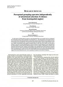
Figure 5: A viewpoint sequence a)..d), taken out of the Monte-Carlo training simulation. From left to right: firstly, the projective views are given; secondly, the planar graphs; thirdly, the Bayes’ belief networks, showing trigram-realizations and their bigram replacements (i.e. up to three conditional variables are possible, when using trigrams, shown in red colored nodes); hence, if it is possible to get a ’cheaper’ junction conditioning with bigrams, the belief networks are restructured to appear only in two conditional variables at maximum.
10
and especially understanding of unknown complex objects will become feasible. From this work, it follows that the combination of both, the planar graph representation proposed in [6], and the statistical approach of grammatical inference by a N-gram model of this work, performs better than the subgraph matching approach proposed in [7], if they are compared in terms of runtime complexity and learning efficiency. However, as simple as humans may investigate an unknown object in order to understand its topology, the approach supports such a investigation by combining a sequence of images from different viewpoints for learning of implicit object topology.
Acknowledgment This work was supported by project S9101 ”Cognitive Vision” of the Austrian Science Foundation. The authors would like to thank Mrs. Fariba Dehghani-Schobesberger for the fruitful discussions on the topic of this work.
References [1] F. Ackermann, A. Maßmann, S. Posch, G. Sageder, and D. Schl¨ uter. Perceptual grouping of contour segments using markov random fields. Patt. Rec. and I. A., 7(1):11–17, 1997. [2] I. Biederman. Recognition by components. Psych. Rev., 94, 1987. [3] C. G. Christou, B. S. Tjan, and H. H. B¨ ulthoff. Viewpoint information provided by a familiar environment facilitates object identification. TR Max-Planck institute f. biol. cybernetics., 68, 1999. [4] O. Faugeras. Three-Dimensional Computer Vision. MIT Press., 2001. [5] M. A. Fischler and R. C. Bolles. Random sample consensus: A paradigm for model fitting. Comm. of the ACM., 24(9):381–395, 1981. [6] P. M. Goebel and M. Vincze. A cognitive modeling approach for the semantic aggregation of object prototypes from geometric primitives. In Proc. ACIVS, Delft Univ. (NL), 2007. [7] P. M. Goebel and M. Vincze. Implicit modeling of object topology with guidance from temporal view attention. In Proc. of ICVW 2007, Bielefeld University (D), 2007. [8] P. M. Goebel and M. Vincze. Vision for cognitive systems: A new compound concept connecting natural scenes with cognitive models. In LNCS, INDIN 07, Austria., 2007. [9] R. M. Haralick and L. G. Shapiro. Image segmentation techniques. Computer Vision, Graphics and Image Processing., 29(1):100–132, January 1985. 11
[10] C. Higuera. Data Complexity in Pattern Recognition, Eds. M. Basu and Tin Kam Ho., chapter Data Complexity Issues in Grammatical Inference . Prentice Hall., 2006. [11] D. Jurafsky and J. H. Martin. Speech and Language Processing: An Intro. to Natural Language Processing, Comp. Linguistics and Speech Recognition. Prentice Hall., 2003. [12] C. Kermorvant and P. Dupont. Stochastic grammatical inference with multinomial tests. In ICGI ’02: Proc. on Grammatical Inf. Springer, 2002. [13] K. Koffka. Principles of Gestalt Psychology. Hartcourt, NY, 1935. [14] A. Levinshtein, C. Sminchisescu, and S. Dickinson. Learning hierarchical shape models from examples. In Proc. EMMCVPR 2005, 2005. [15] D. G. Lowe. Three-dimensional object recognition from single two-dimensional images. Artificial Intelligence., 31(3):335–395, 1987. [16] D. Marr. Vision: A Computational Approach. Freeman & Co., 1982. [17] S. Procter. Model-Based Polyhedral Object Recognition Using Edge-Triple Features. PhD thesis, Centre for Vision, Speech and Signal Processing, University of Surrey, UK., 1998. [18] S. Sarkar. and K. L. Boyer. Integration, inference, and management of spatial information using bayesian networks. IEEE Trans. Patt. Anal. and M. Intell., 15(3):256–274, 1993. [19] S. Sarkar. and K. L. Boyer. Perceptual organization in computer vision: A review and a proposal for a classificatory structure. IEEE Trans. on Systems, Man, and Cybernetics., 23(2):382–399, 1993. [20] W. St¨ocher and G. Biegelbauer. Automated simultaneous calibration of a multi-view laser stripe profiler. In ICRA ’05: Proc. of IEEE Int. Conf. on Rob. and Aut., 2005. [21] R. F. Wang and E. S. Spelke. Human spatial representation: insights from animals. Trends in Cognitive Sciences., 6(9), 2002. [22] A. Witkin and J. Tenenbaum. On the role of structure in vision, in human and machine vision. In Proc. Conf. on Human Vision., pages 481–543. Acad. Press Inc., 1983. [23] M. Zillich. Making sense of images: Parameter-free perceptual grouping. PhD thesis, ACIN, Automation & Control Institute, Vienna University of Technology., 2007. [24] S. W. Zucker. Vision, Brain, and Cooperative Computation (M.A. Arbib and A.R. Hanson, Eds.), pages 231–262. Cambridge, MA: MIT Press., 1987.
12