Linear Feature Extraction Using Perceptual Grouping And Graph-Cuts Charalambos Poullis CGIT/IMSC, USC Los Angeles, CA 90089
[email protected]
Suya You
CGIT/IMSC, USC Los Angeles, CA 90089
[email protected]
ABSTRACT In this paper we present a novel system for the detection and extraction of road map information from high-resolution satellite imagery. Uniquely, the proposed system is an integrated solution that merges the power of perceptual grouping theory (gabor filtering, tensor voting) and segmentation (graph-cuts) into a unified framework to address the problems of road feature detection and classification. Local orientation information is derived using a bank of gabor filters and is refined using tensor voting. A segmentation method based on global optimization by graph-cuts is developed for segmenting foreground(road pixels) and background objects while preserving oriented boundaries. Road centerlines are detected using pairs of gaussian-based filters and road network vector maps are finally extracted using a tracking algorithm. The proposed system works with a single or multiple images, and any available elevation information. User interaction is limited and is performed at the begining of the system execution. User intervention is allowed at any stage of the process to refine or edit the automatically generated results.
1.
INTRODUCTION
Traditional road mapping from aerial and satellite imagery is an expensive, time-consuming and labor-intensive process. Human operators are required at every part of the process to mark the road map in the images. In recent research, several computer vision based systems were proposed for the semi-automated or automated road map extraction. However, the gap between the state of the art and the goal still remains wide. Currently, there is no existing method which allows for the complete and reliable extraction of road map information from aerial and satellite imagery. Hence, there is still a need for an automated procedure that can reliably and completely detect and extract road networks and update road databases in Geospatial Information Systems. In this work, we propose an integrated system for the automatic detection and extraction of road networks from aerial
Ulrich Neumann
CGIT/IMSC, USC Los Angeles, CA 90089
[email protected]
and satellite images. To our best knowledge, there is no work done in combining perceptual grouping theories and segmentation using graph-cuts for the automatic extraction of road feature. Gabor filters tuned at varying orientations and frequencies are used to extract features of special interest. A tensorial representation which allows for the encoding of multiple levels of structure information(points, curves, surfaces) for each point is used to represent the features extracted by the filters. Such a representation is very efficient when dealing with noisy, incomplete and complicated scenes. The classification of the encoded features is then based on a tensor voting communication process that is governed by a perceptual field, encoding the constraints and rules of how a point receives/casts votes from/to its neighbors. The accumulation of votes at each point provides an accurate estimate of the features going through the point (Section 3). An orientation-based segmentation using graph-cuts is used to segment the road candidates using the refined feature information resulting from the tensor voting process (Section 4). The road centerlines are then detected using a pair of bi-modal and single mode gaussian-based kernels which respond to parallel lines and flat areas respectively. Finally, a tracking algorithm is used to extract the road network vector map (Section 5).
2.
BACKGROUND AND RELATED WORK
Several techniques have been proposed and developed so far and can be separated into three main categories: pixelbased, region-based and knowledge-based.
2.1
Pixel-based
Edge detection. The goal of edge detection is to find at which points in the image the intensity value changes sharply. Although, many edge detectors [4, 15, 14, 6] already exist, none of them can extract complete road segments from a given image. Instead, the output is a list of possible edge points which have to be processed further. In [1] lines are extracted in an image with reduced resolution as well as roadside edges in the original high resolution image. Similarly, [11] uses a line detector to extract lines from multiple scales of the original data. [17] applies Steger’s differential geometry approach [16] for the line extraction. Road detection. Road detection is performed using a model of a road or a modified edge detector. The goal is to detect the roads as parallel lines separated by a constant
width. In [10] they use a multi-scale ridge detector [16] for the detection of lines at a coarser scale, and then use a local edge detector [4] at a finer scale for the extraction of parallel edges. Linking the two edges together, creates a ”ribbon”, which is then optimized using a variation of the active contour models technique-snakes introduced by [9].
type passing from that point x. A tensor T is defined as, 32 T 3 2 ~e1 0 ˆ ˜ λ1 0 T = ~e1 ~e2 ~e3 4 0 λ2 0 5 4 ~eT2 5 (1) 0 0 λ3 ~eT3
T = λ1~e1~eT1 + λ2~e2~eT2 + λ3~e3~eT3
2.2
Region-based
The goal of the region-based techniques is to segment the image into clusters using classification or region-growing algorithms. In [19] they use predefined membership functions for road surfaces (spectral signature, reflectance properties) as a measure for the image segmentation and clustering. Likewise, in [5] they use the reflectance properties, from the ALS data and perform a region growing algorithm to detect the roads. [8] uses a hierarchical network to classify and segment the objects.
2.3
Knowledge-based
Knowledge can have several forms. In [17], human input is used to guide a system in the extraction of context objects with associated confidence measures. A similar approach is used for context regions where rural areas are extracted from the SAR images and a weight is assigned to each region. The system in [18] integrates knowledge processing of color image data and information from digital geographic databases, extracts and fuses multiple object cues, thus takes into account context information, employs existing knowledge, rules and models, and treats each road subclass accordingly. [5] uses a rule-based algorithm for the detection of buildings at a first stage and then at a second stage the reflectance properties of the road. Explicit knowledge about geometric and radiometric properties of roads is used in [17] to construct road segments from the hypotheses of roadsides.
3. PERCEPTUAL GROUPING 3.1 Gabor Filtering We employ a bank of gabor filters tuned at 8 different orientations θ linearly varying from 0 ≤ θ < π, and at 5 different high-frequencies(per orientation) for multi-scale analysis. The remaining parameters of the filters are computed as functions of the orientation and frequency parameters as in [7]. The filtered images are then grouped according to the orientation of the filters, thus resulting in 8 images; one per orientation. The higher the response of a point in an image, the more likely that the feature at that point is aligned to the direction of the filter used to produce the image and vice-versa. Finally, all pixels in the resulting 8 images are encoded into tensors as explained in the next section.
3.2
Tensor Voting Overview
Tensor voting is a perceptual grouping and segmentation framework introduced by [13]. The data representation is based on tensor calculus and the communication of the data is performed using linear tensor voting. In this framework, a point x ∈ R3 is encoded as a second order symmetric tensor which captures the geometric information for multiple feature types(junction, curve, surface) and a saliency, or likelihood, associated with each feature
(2)
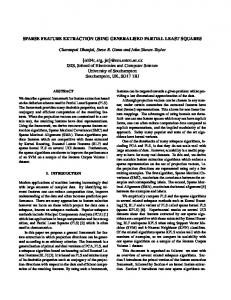
where λ1 ≥ λ2 ≥ λ3 ≥ 0 are eigenvalues, and ~e1 , ~e2 , ~e3 are the eigenvectors corresponding to λ1 , λ2 , λ3 respectively. By applying the spectrum theorem, the tensor T in equation 2 can be expressed as a linear combination of three basis tensors(ball, plate and stick) as in equation 3. T = (λ1 −λ2 )~e1~eT1 +(λ2 −λ3 )(~e1~eT1 +~e2~eT2 )+λ3 (~e1~eT1 +~e2~eT2 +~e3~eT3 ) (3) In equation 3, (~e1~eT1 ) describes a stick(surface) with associated saliency (λ1 − λ2 ) and normal orientation ~e1 , (~e1~eT1 + ~e2~eT2 ) describes a plate(curve) with associated saliency (λ2 − λ3 ) and tangent orientation ~e3 , and (~e1~eT1 +~e2~eT2 +~e3~eT3 ) describes a ball(junction) with associated saliency λ3 and no orientation. The geometrical interpretation of tensor decomposition is shown in Figure 1(a). Every point in the images
(a) 3D Tensor decom- (b) Votes casting. (c) Example position. result Figure 1: (a)Tensor decomposition,(b)vote casting,(c)Before (left) and after (right) the tensor voting.. computed previously is encoded using equation 1 into a unit plate tensor with its orientation ~e3 aligned to the filter’s orientation and is scaled by its response in the filtered image, therefore giving 8 differently oriented tensors per point. Adding the 8 tensors of each point gives a tensor describing the feature types passing through that point. The tensor encoded points then cast a vote to their neighbouring points which lie inside their voting fields, thus propagating and refining the information they carry(Figure 1(b)). For a comprehensive analysis and further details refer to [13]. Figure 1(c) shows the test image with an incomplete polygon in white and the resulting curves being overlaid in yellow. As it is obvious, most of the discontinuities were succesfully and accurately recovered by this process. A process which combines the local precision of the gabor filters with the global context of tensor voting is performed, as a series of sparse and dense votings similarly to [12]. Finally, by analyzing the information encoded in the tensors the most dominant feature type of each point is determined as the feature type with the highest associated likelihood(i.e.
λ1 −λ2 , λ2 −λ3 , λ3 in equation 3). The classified curve points with their associated orientation information computed are then used to guide the orientation-based segmentation process.
4.
ORIENTATION-BASED SEGMENTATION USING GRAPH-CUTS
The result is a segmented foreground image consisting of road candidate points, and a background image consisting of non-road and vegetation points.
4.1
Graph-cut Overview
In [3, 2] the authors interpret image segmentation as a graph partition problem. Given an input image I, an undirected graph G =< V, E > is created where each vertex vi ∈ V corresponds to a pixel pi ∈ I and each undirected edge ei,j ∈ E represents a link between neighbouring pixels pi , pj ∈ I. In addition, two distinguished vertices called terminals Vs , Vt , are added to the graph G. An additional edge is also created connecting every pixel pi ∈ I and the two terminal vertices, ei,Vs and ei,Vt . For weighted graphs, every edge e ∈ E has an associated weight we . A cut C ⊂ E is a partition of the vertices V of the graph G into two disjoint sets S,T where Vs ∈ S and Vt ∈ T . The cost of each cut C is the sum of the weighted edges e ∈ C. The minimum cut problem can then be defined as finding the cut with the minimum cost which can be achieved in near polynomial-time [3]. The binary case can easily be extended to a case of multiple terminal vertices. We create two terminal vertices for foreground O and background B pixels for each orientation θ for which 0 ≤ θ ≤ π. In our experiments, we have found that choosing the number of orientation labels in the range Nθ = [2, 8] generates visually acceptable results. Thus the set of labels L has size |L| = 2 ∗ Nθ and is defined to be L = {Oθ1 , Bθ1 , Oθ2 , Bθ2 ..., OθNθ , BθNθ }
4.2
Energy minimization function
Finding the minimum cut of a graph is equivalent to finding an optimal labeling f : Ip −→ L which assigns a label l ∈ L to each pixel p ∈ I where f is piecewise smooth and consistent with the original data. Thus, our energy function for the graph-cut minimization is given by E(f ) = Edata (f ) + λ ∗ Esmooth (f )
∆p,q = ² +
1 + (Ip − Iq )2 1 + (θp − θq)2
(6)
The above function favors towards neighbouring pixels with similar intensities and orientations and penalizes otherwise. In addition, we define a measure of smoothness for the global minimization. Let If (p) and If (q) be the intensity values under a labeling f . Similarly, let θf (p) and θf (q) be the orientations under the same labeling. We define a measure of the smoothness between neighbouring pixels p, q under a labeling f as 1 + (If (p) − If (q) )2 ∆˜p,q = ² + 1 + (θf (p) − θf (q) )2
(7)
Using the smoothness measure defined for the observed data and the smoothness measure defined for any given labeling we can finally define the energy smoothness term as follows, X Kp,q ∗ ∆˜p,q (8) Esmooth (f ) = {p,q}∈N −
∆2 p,q
where N is the set of neighbouring pixels, Kp,q = [e 2∗σ2 ], ² is a small positive constant and σ controls the smoothness uncertainty. The energy function E(f ) penalizes heavily for severed edges between neighbouring pixels with similar intensity and orientation, and vice versa, which results in better defined boundaries as shown in the comparison presented in Figure 2.
(a) Original (b) Intensity- (c) (d) Differimage. based. Orientation- ence image based. Figure 2: Comparison between intensity- and orientation-based segmentation.Difference image color codes - (red: common points, green: only in inten. segm., blue: only in orient. segm.)
(4)
where λ is the weight of the smoothness term. Energy data term. The data term provides a per-pixel measure of how appropriate a label l ∈ L is, for a pixel p ∈ I in the observed data and is given by, X Edata (f ) = Dp (fp ) (5) p∈I
where Dp (fp ) = ² +
of the observed smoothness between pixels p and q as
1−ln(P (Ip |f (p))) . 1+(θp −θf (p) )2
Energy smoothness term. The smoothness term provides a measure of the difference between two neighbouring pixels pi , pj ∈ I with labels li , lj ∈ L respectively. Let Ip and Iq be the intensity values in the observed data of the pixels p, q ∈ I respectively. Similarly, let θp and θq be the initial orientations for the two pixels. We define a measure
5. ROAD EXTRACTION 5.1 Parallel-line Detection A bi-modal gaussian-based filter is applied on the curve saliency map returned by the tensor voting to detect parallellines. In order to ensure that the parallel-lines correspond to road sides a single mode gaussian-based filter is applied on the segmented road pixels(binary image). This ensures that the area between the parallel-lines is part of a road and not a false positive for example, a road-side and a building’s boundary along the side of the road. Three types of information is extracted for each point: the maximum response at each point and, the orientation and width corresponding to the maximum response. This information is then used by the road tracking algorithm to form road segments.
5.2
Road Tracking
Starting from a centerline pixel the road tracking algorithm recursively connects the best neighbouring match. The best match is determined based on the magnitude, orientation and width differences. The result is a set of connected road segments which are finally merged and converted to a vector map.
6.
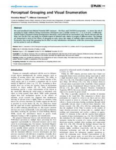
(a) Orientation-based segm.
(b) Centerline sponse(automatic).
re-
(c) Connected centerline components(automatic).
(d) Refined connected centerline components(interactive).
(e) Tracked road segments.
(f) Vector data
EXPERIMENTAL RESULTS
In our experiments, the smoothness term in 4 was set as λ = 0.25 and the number of orientation labels used Nθ = 8.
(a) Original
(c) Centerline traction
(b) Orientationbased segmentation
ex-
(d) Extracted network
road
Figure 3: Automatic mode(No user intervention),High resolution satellite image of an urban site with no additional elevation information. In (a),(b) the marked areas show occlusions and shadows.
7.
REFERENCES
[1] A. Baumgartner, C. T. Steger, H. Mayer, W. Eckstein, and H. Ebner. Automatic road extraction in rural areas. In ISPRS Congress, pages 107–112, 1999. [2] Y. Boykov and M.-P. Jolly. Interactive graph cuts for optimal boundary and region segmentation of objects in N-D images. In ICCV, pages 105–112, 2001. [3] Y. Boykov, O. Veksler, and R. Zabih. Fast approximate energy minimization via graph cuts. In ICCV, pages 377–384, 1999. [4] J. Canny. A computational approach to edge detection. In RCV87, pages 184–203, 1987. [5] S. Clode, F. Rottensteiner, and P. Kootsookos. Improving city model determination by using road detection from lidar data. In IAPRSSIS Vol. XXXVI - 3/W24, pp. 159-164, Vienna, Austria, 2005. [6] R. Deriche. Using canny’s criteria to derive a recursively implemented optimal edge detector. Inter. J. Computer Vision, 1(2), May 1987. [7] I. R. Fasel, M. S. Bartlett, and J. R. Movellan. A comparison of gabor filter methods for automatic detection of facial landmarks. In ICAFGR, pages 231–235, 2002. [8] P. Hofmann. Detecting buildings and roads from ikonos data using additional elevation information. In Dipl.-Geogr. [9] M. Kass. Snakes: Active contour models. Inter. J. Computer Vision, 1(4):321–331, 1980. also in ICCV1, 1987. [10] I. Laptev, H. Mayer, T. Lindeberg, W. Eckstein, C. Steger, and A. Baumgartner. Automatic extraction of roads from
Figure 4: Interactive mode. (a) Segmentation result. (b) Automatic extraction of centerline information. (c) The centerline components recovered automatically. (d) The user refined centerline components. (e) The tracked road segments automatically computed using (d). (f ) The final road map vector data.
[11]
[12]
[13] [14] [15] [16] [17] [18] [19]
aerial images based on scale space and snakes. Mach. Vis. Appl, 12(1):23–31, 2000. G. Lisini, C. Tison, D. Cherifi, F. Tupin, and P. Gamba. Improving road network extraction in high-resolution sar images by data fusion. In CEOS SAR Workshop 2004, 2004. A. Massad, M. Bab´ os, and B. Mertsching. Perceptual grouping in grey-level images by combination of gabor filtering and tensor voting. In ICPR (2), pages 677–680, 2002. G. Medioni, M. S. Lee, and C. K. Tang. A Computational Framework for Segmentation and Grouping. Elsevier, 2000. K. K. Pingle. Visual perception by a computer. In Automatic Interpretation and Classification of Images, pages 277–284, 1969. L. G. Roberts. Machine perception of 3-D solids. In Optical and Electro-Optical Info. Proc., pages 159–197, 1965. C. Steger. An unbiased detector of curvilinear structures. Technical Report FGBV-96-03, Technische Universit¨ at M¨ unchen, M¨ unchen, Germany, July 1996. B. Wessel. Road network extraction from sar imagery supported by context information. In ISPRS Proceedings, 2004. C. Zhang, E. Baltsavias, and A. Gruen. Knowledge-based image analysis for 3d road construction. In Asian Journal of Geoinformatic 1(4), 2001. Q. Zhang and I. Couloigner. Automated road network extraction from high resolution multi-spectral imagery. In ASPRS Proceedings, 2006.