Perceptual image attribute scales derived from overall image quality

Perceptual image attribute scales derived from overall image quality assessments Kyung Hoon Oh, Sophie Triantaphillidou, Ralph E. Jacobson Imaging Technology Research Group, University of Westminster, Harrow, UK

ABSTRACT Psychophysical scaling is commonly based on the assumption that the overall quality of images is based on the assessment of individual attributes which the observer is able to recognise and separate, i.e. sharpness, contrast, etc. However, the assessment of individual attributes is a subject of debate, since they are unlikely to be independent from each other. This paper presents an experiment that was carried to derive individual perceptual attribute interval scales from overall image quality assessments, therefore examine the weight of each individual attribute to the overall perceived quality. A psychophysical experiment was taken by fourteen observers. Thirty two original images were manipulated by adjusting three physical parameters that altered image blur, noise and contrast. The data were then arranged by permutation, where ratings for each individual attribute were averaged to examine the variation of ratings in other attributes. The results confirmed that one JND of added noise and one JND of added blurring reduced image quality more than did one JND in contrast change. Furthermore, they indicated that the range of distortion that was introduced by blurring covered the entire image quality scale but the ranges of added noise and contrast adjustments were too small for investigating the consequences in the full range of image quality. There were several interesting tradeoffs between noise, blur and changes in contrast. Further work on the effect of (test) scene content was carried out to objectively reveal which types of scenes were significantly affected by changes in each attribute. Keywords: Psychophysical scaling, image quality, overall quality assessment, perceptual quality attributes.

1.

INTRODUCTION

Image quality can be defined as the overall impression of image excellence. Many psychophysical investigations have been conducted on the assessment of individual image attributes. This individual assessment has been the subject of discussion since a single image quality attribute is unlikely to be independent from other attributes [1, 2]. It creates a problem in simplifying image quality measurements since it does not consider the complicated relationships between them [3]. This paper describes experimental work that was carried out to derive individual perceptual attribute interval scales from overall image quality assessments. This approach does not require scaling of individual attributes and does not require the assumption that the attribute is one dimensional. This research aims: 1) to investigate the perceptual constraints that determine image quality 2) to determine the weight of each individual attribute to the overall image quality.

2.

IMPLEMENTATION OF PSYCHOPHYSICAL SCALING

2.1 Image acquisition and selection Images of natural scenes were acquired i) by image capture, using a digital camera and ii) from two Master Kodak Photo CDs, to cover a range of images with differing content and characteristics. The scenes represented a variety of subjects, such as portraits, natural scenes, buildings with plain and busy background, etc. They were chosen to include various global and local illuminations, numerous colours, varying number and strength of lines, edges and spatial distribution of the subjects. The test scenes are included in Appendix.

Fifteen natural scenes were captured using a Canon EOS-1Ds full frame digital SLR camera, equipped with a Canon EF 28-135mm f 3.5-5.6 IS USM zoom lens. The ISO 100 setting was used to capture all scenes. Camera exposure was determined by taking multiple reflection readings from various parts of the scene. This was achieved with the throughthe-lens centre-weighting and spot metering modes of the camera. The camera was set to auto colour balance mode and sRGB colour mode. The lens was focused manually. Scenes were recorded at about 11 mega pixels resolution (4064 × 2704) in a CMOS sensor (with approximately 8.8 µm square pixel dimensions). The scenes were saved as 12-bit RAW files and then downloaded to a computer as 8-bit TIFF uncompressed images by using the software provided by Canon, via an IEEE 1394 connection. In addition seventeen natural scenes were selected from two Master Kodak Photo CDs. The Master Kodak Photo CD images were opened at a spatial resolution of 512 by 786 and at a colour resolution of 8 bits per channel. All thirty two images were down-sampled to 317 by 476 pixels using spline interpolation and saved as TIFF files of approximately 400 KB. 2.2 Test Stimuli The thirty two original images were manipulated by altering three physical parameters: Gaussian blurring, Gaussian noise and contrast adjustment to obtain a large number of test stimuli with different levels of blur, noise and contrast. Prior to deciding the ranges and levels of distortion, pilot studies were conducted on the calibrated 21 inch EIZO CG-210 LCD, which was then used for the investigation. Each chosen distortion level corresponded to approximately one JND when images were viewed on the display. The following techniques were chosen for the manipulation of the original stimuli: Blurring: Firstly, Gaussian blurring was applied on the thirty two originals. The standard deviation (σ) of the Gaussian low-pass kernel ranged from 0.01 to 1.24 at 0.3075 intervals. This created a total of one hundred and sixty test images. Additive Noise: After blurring, the images were further distorted by Gaussian noise filtering, using three different standard deviations (σ): 0.0, 0.1 and 0.2. This function created three different levels of uniform noise and provided a total of four hundred and eighty distorted images. Contrast adjustment: After blurring and adding noise, contrast adjustment was applied to all distorted images at five different levels. This included the original level, two levels for contrast enhancement and two levels for contrast reduction. The five levels of contrast were achieved by varying contrast (γ) from 0.9 to 1.1, at 0.05 intervals. A total of two thousand four hundreds test stimuli were finally created. 2.3 Psychophysical display, interface and viewing conditions Psychophysical tests were carried out under dark viewing conditions. All images were displayed on an EIZO CG-210 LCD, controlled by the S3 Graphics Prosavage DDR graphic card in a personal computer. The graphic card was configured to display 24-bit colour, at a resolution of 1600 by 1200 pixels and a frequency of 60 HZ. The display was switched on for fifteen minutes before the tests to allow stabilization. It was placed at a viewing distance of approximately 60 cm from the observers, and subtended a visual angle of roughly 10o. The Eye-One Pro monitor calibrator was used to calibrate the display at a white point close to D65, a contrast of 2.2 and a white point luminance of 100 cd/m2 – the default settings for contrast and luminance for this monitor. 2.4 Observations Subjective assessments were performed by a panel of fourteen selected observers, seven males and seven females. They were all familiar with the meaning and assessment of image quality. The age of observers ranged from 21 to 52 years old. All observers had normal colour vision and normal or corrected-to-normal visual acutance. Each observer undertook a categorical scaling experiment 6 times, each time evaluating a different set of images. Each

individual observation period was around 45 minutes. The standard ISO20462-1 suggests that the observation periods should be a maximum of 60 minutes to avoid tiredness or lack in concentration [4]. Before starting the test, observers were allowed several minutes to adapt to the dark viewing conditions of the laboratory [5]. Images were displayed one at a time, randomly, in the centre of the display area to minimise non-uniformity display effects. Observers were asked to place each test image according to the perceived image quality in one out of 5 quality categories, with 1 indicating the worst quality and 5 the best quality.

3.

ANALYSIS OF THE ASSESSMENTS

3.1 Scaling overall image quality Interval scales were derived using the simplest condition, D, of Torgerson’s Law of Categorical Judgements [6], which makes minimum assumptions regarding the category and sample variance: correlation coefficients and dispersions of both the sample and the category are constant. Category boundaries and sample values were obtained. The least square technique was applied to prevent inaccurate scale values from zero-one elements in proportion matrix [6].

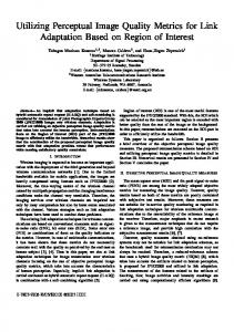
Figure 1. Interval scales of combined scenes

Figure 1 presents interval scales of overall image quality from the combined (average of) 32 scenes. Each label in the x axis represents a specific level of distortion - in blurring (B) and noise (N). Within each of these levels there are 5 different variations in contrast - represented by the individual points in the graph. Each label corresponds to the point which indicates the 1st variation in contrast (i.e. therefore C1 in the label). The results confirmed that the modifications in all three image attributes, in most cases, decreased image quality. The original versions of the images had an average scale value of 2.03, whilst most of the distorted images had a lower scale value. The specific changes in contrast did not significantly affect image quality (in a few cases they improved it), while noisiness and sharpness were found to be by far the most influential attributes on perceived image quality. This will be discussed in more detail in the individual attributes scales presented later. The results also indicate scene dependency. The broken lines in Figure 1 indicate the range of scale values derived from all scenes for each level of distortion; the grey square is the average from all scenes.

3.2 Scaling of individual attributes The collected scale values were rearranged using permutation1 [7]. Since we have variations in three different image attributes (i.e. in blurring level, noise level, and contrast) the attributes were first arranged as listed in Step1 of Table 1. The total number of permutations is produced by the product of the total number of distorted images and the number of attribute permutation: 14400 total permutations = (2400 test images) x (6 attribute permutations) The full implementation of the method is illustrated in Table 1. In addition, an example of the implementation is shown in Table 2. The scale values of the individual image attributes were examined across the average (calculated by the mean) scale values of the other attributes [8]. The first listed attribute in Step 1, in Table 1, is the targeting attribute in the permutation. The mean scale value for this attribute is calculated by Steps 2 and 3. Step two calculates the average scale value across the last attribute listed in Step 1, Table 1. Step 3 calculates the average scale value across the last listed attribute in Step 2, Table 1. Step 1: Arrangement

I. II. III. IV. V. VI.

5 blur 5 blur 3 noise 3 noise 5 contrast 5 contrast

3 noise 5 contrast 5 contrast 5 blur 5 blur 3 noise

Step 2: Average of last column in Step 1

5 contrast 3 noise 5 blur 5 contrast 3 noise 5 blur

I. II. III. IV. V. VI.

5 blur 5 blur 3 noise 3 noise 5 contrast 5 contrast

Step 3. Average of last column in Step 2

3 noise 5 contrast 5 contrast 5 blur 5 blur 3 noise

I. II. III. IV. V. VI.

5 blur 5 blur 3 noise 3 noise 5 contrast 5 contrast

Table 1. Individual attribute scaling Step 1 Attributes

I

Blur1Noise1Contrast1 Blur1Noise1Contrast2 Blur1Noise1Contrast3 Blur1Noise1Contrast4 Blur1Noise1Contrast5 Blur1Noise2Contrast1 Blur1Noise2Contrast2 Blur1Noise2Contrast3 Blur1Noise2Contrast4 Blur1Noise2Contrast5 Blur1Noise3Contrast1 Blur1Noise3Contrast2 Blur1Noise3Contrast3 Blur1Noise3Contrast4 Blur1Noise3Contrast5

Scale value 1.47 1.79 1.79 1.73 1.42 1.15 1.79 0.96 1.68 1.52 1.08 1.22 1.38 1.15 0.8

Step 2 Attributes

Scale value

Blur1Noise1

1.64

Blur1Noise2

1.42

Blur1Noise3

1.13

Step 3 Attributes Scale value

Blur1

1.39

Table 2. Example of individual attribute scaling

1

Permutation means arrangement of items. The word arrangement is used, if the order of items is considered. In general, the number of permutation is taken by nPr , where n is different item of r at a position. Three of stimuli and three at a time forms six permutations, 3 P3.=3!= 6.

Results from cases I to VI from Step 1, Table 1, are shown in Figure 2. Each resulting figure uses the same data, but they are presented differently i.e. according to the targeting attribute (listed first in the title of the graph), then the second and third attributes. For example the top left graph in Figure 2 presents the data in the same fashion as Figure 1 – case I. In the graph next to it, the data are presented according to the same targeting attribute but the second and third attributes are interchanged – case II. The middle row in Figure 2 shows cases III and IV and the last row cases V and VI, as listed in Table 1. Similarly to Figure 1, on the graphs on Figure 2 the labels in the x axis represent a specific level of distortion for the targeting and second attributes, where as each point represents the scale value of the targeting, second and third attributes. Further results from Step 2, Table 1, are shown in Figure 3. Finally, the individual attribute scales are presented in Figure 4, which are derived from the final Step 3 in the process. The results present the mean scale value of quality for each attribute.

Figure 2. Resulting scales from Step 1

There are several interesting tradeoffs in image quality when varying the three attributes, i.e. blur, noise and contrast (Figure 3). The results agrees with previous research which found that the higher the sharpness the higher the graininess [8, 9]. This is observed in Figure 3, cases I and IV (Blur-Noise & Noise-Blur) which indicate that high amount of blur in the image significantly decreased the perception of noise (case I) and high noise decreased perceived blur (case IV). The relationship between the contrast and the other attributes is not significant for the specific levels of contrast modification that were used for this experiment, which appear not to have altered image quality. This is seen in Figure 4 which indicates that one JND of added noise and one JND of blur reduced image quality much more than one JND in contrast changes.

Figure 3. Interval scales of combined scenes (Step 2)

From Figure 4, adding noise reduces the quality scale values by an average of 0.48, adding blur also reduced it by an average of 0.41, whereas increasing contrast increased it very slightly by 0.01. Case (Blur) we notice that the original and original + 1 JND of blur were almost rated similarly. The quality is shown to decrease significantly for the next blur levels and it reaches a point (at level B5) where more blur would not further reduce it. I.e. the image quality scale of blurring is a hyperbolic (S-shape) function. The ranges of added noise (2 levels) and contrast adjustments (4 levels) were too small for investigating the consequences in the full range of image quality. Case (Noise) indicates that 2 levels of added noise (each separated by 1 JND) decreased equally image quality but the ‘toe’ of the quality scale for noise was not reached. Finally, as mentioned above, 2 modifications in contrast around the ‘optimum’ contrast did not alter image quality – Case(Contrast). The results are of course valid for the specific display and viewing conditions.

Figure 4. Individual attribute scales

3.3 Scene dependency in the observations The results show scene dependency caused by the nature of scenes and their inherent properties. This is shown in Figures 5, 6 and 7, where the mean scale value of the distortion level is indicated by the grey square and the range covered by all scenes with the broken lines. When considering image blurring, as the level of distortion increased the scene dependency decreased. Figure 5 indicates that low levels of blurring might affect different scenes in a different manner, but high levels of blurring tend to affect different scenes more equally. On the other hand, Figures 6 and 7 show that the variation from the mean scale value for added noise and variations in contrast appears similar in all levels of distortion. This result suggests that as image quality decreases we found less and less scene dependency but high quality images tend to be rated differently according to their individual scene content.

Figure 5. Scene dependency on blur scale

Figure 6. Scene dependency on noise scale

Figure7. Scene dependency on contrast scale

The effect of individual scenes was examined. To determine the comparability of the results for each individual scene with the average combined rating for all scenes, the scale values of each scene were plotted against the combined mean ratings from all scenes, for each individual attribute [8]. In the example plot shown in Figure 8 for the scene ‘Saules’, the gradients of the lines fitting the data (one for each attribute) represent the compatibility between the range of ratings for each individual scene and that of the combined scenes. If the gradient of the line is one, the range of scale values for the scene is the same as that of the combined scenes for the specific attribute. If the gradient is larger than 1, then the scene has a larger quality range meaning that it is more sensitive than the ‘average scene’ to the changes in the specific attribute. The reverse is true when the gradient is smaller than one. The correlation coefficient lines fitting the data indicates the strength of relationship between them. The constant in the linear relationship indicates whether, overall, the individual scene got better average quality ratings than the average ratings of the combined scenes (positive offset) or the opposite (negative offset).

Figure 8. Scene dependency on the “Saules”

African tree

Baby Bike China town Exercise Formula Glasses Group Human Human2 Human3 Human4 Kids Landscape Landscape2 Landscape3 London Eye London Eye2 Louvre National gallery Old building Plant1 Plant2 Plant3 Plant4 Plant5 Plant6 St. Pauls St. Pauls2 Saules Sungsil Yellow flower

Blurring Gradient Constant

r2

Noisiness Gradient Constant

r2

Contrast Gradient Constant

r2

0.32

-0.02

0.945

1.96

0.00

0.993

0.75

-0.02

1.06

-0.02

0.995

1.06

-0.02

0.995

-1.62

-0.04

0.394 0.460

1.21

0.30

0.984

0.72

0.29

0.994

2.60

0.29

0.954

0.95

0.04

0.995

0.97

0.04

0.984

2.60

0.04

0.764

1.15

-0.20

0.966

0.51

-0.21

0.989

1.37

-0.21

0.442

1.00

0.53

0.997

1.14

0.53

0.978

0.03

0.52

0.000

0.86

0.10

0.974

1.17

0.11

1.000

-2.81

0.09

0.564

1.07

-0.38

0.980

0.66

-0.38

1.000

2.28

-0.38

0.565

0.91

0.07

0.990

1.10

0.06

1.000

1.44

0.06

0.517

0.32

0.31

0.948

1.07

-0.30

0.998

2.13

-0.30

0.589

1.24

-0.20

0.965

0.55

-0.21

0.998

2.09

-0.21

0.764

1.08

-0.43

0.991

1.11

-0.43

0.977

4.28

-0.42

0.946

1.18

0.27

0.996

1.15

0.26

1.000

3.06

0.27

0.589

0.86

-0.20

0.967

1.44

-0.19

1.000

2.03

-0.20

0.761

0.63

0.06

0.936

1.82

0.06

0.976

1.10

0.05

0.871

1.05

0.07

0.987

1.31

0.07

0.999

-0.07

0.06

0.001

0.86

-0.37

0.996

1.09

-0.38

0.989

-0.09

-0.38

0.003

0.93

-0.42

0.999

1.28

-0.41

0.987

-1.12

-0.43

0.444

1.16

-0.35

0.998

1.03

-0.36

1.000

0.10

-0.37

0.014

1.07

-0.13

0.996

0.96

-0.13

1.000

2.40

-0.12

0.469

1.29

0.08

0.997

0.92

0.08

1.000

-0.78

0.07

0.093

1.15

0.79

0.985

0.34

0.79

0.841

2.40

0.80

0.844

0.79

0.53

0.969

0.85

0.53

0.993

5.07

0.54

0.986

0.87

0.22

0.992

1.13

0.21

0.997

-1.50

0.20

0.353

0.80

-0.12

0.994

1.12

-0.12

0.991

-1.53

-0.13

0.607

1.09

0.08

0.998

0.99

0.08

0.988

0.59

0.07

0.168

0.97

0.13

0.997

1.04

0.13

1.000

-1.32

0.11

0.350

1.40

0.03

0.991

0.50

0.02

0.999

3.06

0.03

0.851

1.10

0.03

0.996

0.87

0.03

0.999

-1.47

0.01

0.480

1.43

0.01

0.964

0.19

0.00

0.861

0.09

0.00

0.001

1.24

-0.31

0.981

0.83

-0.31

0.990

2.66

-0.31

0.857

0.91

0.23

0.996

1.14

0.22

0.989

-0.01

0.22

0.001

Table 3. The gradient, constant, and correlation coefficients for each test image for all 3 attributes

Table 3 presents the gradient, constant and correlation coefficient of the regression lines for each test scene and for all three attributes. Regarding blurring: the scenes “Human2”, “African tree” and “Landscape2” were found to be the three less sensitive scenes to blurring, with the lower gradient values. On the other hand, “Saules” has the highest gradient value, indicating high sensitivity to blurring. Regarding added noise: An extreme result was produced by the “Saules” scene (Figure 8), which was shown the most insensitive scene to added noise, having an extremely low gradient of 0.19. This is the busiest scene in the set [10] and the noise was probably masked by the high frequency information in this scene. The most unusual results regarding both blurring and noise were produced from the “African tree” scene. The scene was found to be the most sensitive to added noise (gradient = 1.96) and the second most insensitive to blurring (gradient = 0.32). This result was also confirmed by previous research [11]. The correlation coefficients of the linear regression on blurring and added noise were all close to 1.0 whereas on contrast they were variable (0.001~0.9861).

4.

CONCLUSION

A large-scale categorical judgment experiment was conducted. In all 14 observers performed a total of 2400 observations. Psychometric scaling was used to create interval scales indicating the quality of images subjected to blur, noise and variations in contrast. This work successfully derived individual perceptual attribute interval scales from overall image quality assessments and the following summary lists the main effects of the individual attributes. 1. One JND of added noise and one JND of added ‘blurring’ reduced image quality more than one JND in contrast change - in the range of distortion applied in this experiment. 2. The range of distortion was introduced by blurring to cover the entire image quality scale; however, the ranges of added Gaussian noise and contrast adjustment were too small for investigating the consequences on the full range of image quality. 3. Blurring decreased significantly the perception of noise. 4. Adding noise decreased perceived blurring. 5. Image quality assessments showed scene dependency. 6. As image quality decreases we found less and less scene dependency but high quality images tend to be rated differently according to their individual scene content. Further work on the effect of scene content will be carried out to objectively reveal which types of scenes are significantly affected by changes in each attribute.

REFERENCES [1] Triantaphillidou, S., “Aspects of Image Quality in the Digitisation of Photographic Collection,” University of Westminster PhD Thesis, London, (2001). [2] Roufs, A., “Perceptual image quality: concept and measurement,” Philips Journal of Research. 30, 33-38 (1992). [3] Engeldrum, P., “The image quality circle,” [Psychometric Scaling], Imcotek Press, Winchester, 5-18. ch 2 (2000). [4] ISO:20462-1., “Photography-psychophysical experimental methods for estimating image quality,” International Organization : ISO, (2005). [5] Hunt, R., “The effect of daylight and tungsten light adaptation on colour perception,” Journal of the Optical Society of America. 40, 362-371 (1950). [6] Engeldrum, P., “Indirect interval scaling-category scaling methods,” [Psychometric Scaling], Imcotek Press, Winchester,123-138. ch 10 (2000). [7] Stroud, K A (Kenneth Arthur)., “Probability,” [Engineering mathematics], Palgrave, Basingstoke, 1155-1197 (2001). [8] Johnson, G and Fairchild, M., “Sharpness Rule,” IS&T Color imaging Conference, 24-30 (2000). [9] Sawyer, J., “Effect of graineiness and sharpness on perceived print quality,” symposium on photographic image quality, 222-231 (1980). [10] Triantaphillidou, S, Allen, E and Jacobson, R., “Image quality Compression Between JPEG and JPEG 2000 II: Scene dependency, Scene analysis and Classification,” Jornal of Imaging Science and Technology. 51(3), 259-270 (2007). [11] Jenkin, R, Triantaphillidou, S. and Richardson, M., “Effective Pictorial Information Capacity as an Image Quality Metric,” Proc: SPIE/IS&T Electronic imaging 2007: Image quality and system performance. 6494, 0-9 (2007).

Appendix

Test images selected for the experiment