digital video image quality and perceptual coding - CiteSeerX

DIGITAL VIDEO IMAGE QUALITY AND PERCEPTUAL CODING H. R. Wu Royal Melbourne Institute of Technology, Australia

K. R. Rao University of Texas at Arlington, USA

To those who have pioneered, inspired and persevered.

Contents List of Figures

iii

List of Tables

vi

2 Fundamentals of Human Vision and Vision Modeling

1

2.1

Introduction . . . . . . . . . . . . . . . . . . . . . . . . . . . . . . . .

1

2.2

A Brief Overview of the Visual System . . . . . . . . . . . . . . . . .

2

2.3

Color Vision . . . . . . . . . . . . . . . . . . . . . . . . . . . . . . . .

4

2.3.1

Colorimetry . . . . . . . . . . . . . . . . . . . . . . . . . . . .

4

2.3.2

Color Appearance, Color Order Systems, and Color Difference .

8

Luminance and the Perception of Light Intensity . . . . . . . . . . . . .

12

2.4.1

Luminance . . . . . . . . . . . . . . . . . . . . . . . . . . . .

12

2.4.2

Perceived Intensity . . . . . . . . . . . . . . . . . . . . . . . .

14

Spatial Vision and Contrast Sensitivity . . . . . . . . . . . . . . . . . .

17

2.5.1

Acuity and Sampling . . . . . . . . . . . . . . . . . . . . . . .

17

2.5.2

Contrast Sensitivity . . . . . . . . . . . . . . . . . . . . . . . .

18

2.5.3

Multiple Spatial Frequency Channels . . . . . . . . . . . . . .

20

2.5.3.1

Pattern adaptation . . . . . . . . . . . . . . . . . . .

21

2.5.3.2

Pattern detection . . . . . . . . . . . . . . . . . . . .

22

2.5.3.3

Masking and facilitation . . . . . . . . . . . . . . . .

23

2.5.3.4

Nonindependence in spatial frequency and orientation

25

2.4

2.5

i

2.6

2.7

2.8

2.5.3.5

Chromatic contrast sensitivity . . . . . . . . . . . . .

26

2.5.3.6

Suprathreshold contrast sensitivity . . . . . . . . . .

28

2.5.3.7

Image compression and image difference . . . . . . .

31

Temporal Vision and Motion . . . . . . . . . . . . . . . . . . . . . . .

32

2.6.1

Temporal CSF . . . . . . . . . . . . . . . . . . . . . . . . . .

32

2.6.2

Apparent Motion . . . . . . . . . . . . . . . . . . . . . . . . .

35

Visual Modeling . . . . . . . . . . . . . . . . . . . . . . . . . . . . . .

37

2.7.1

Image and Video Quality Research . . . . . . . . . . . . . . . .

38

Conclusions . . . . . . . . . . . . . . . . . . . . . . . . . . . . . . . .

39

Index

46

ii

List of Figures 2.1

Maxwell diagram representing the concept of color-matching with three primaries, R, G, and B. . . . . . . . . . . . . . . . . . . . . . . . . . .

5

The CIE 1931 2◦ Standard Observer System of Colorimetry. A) (Top left) The color-matching functions based on real primaries R, G, and B. B) (Top right) The transformed color-matching functions for the imaginary primaries, X, Y,and Z. C) (Bottom) The (x, y) chromaticity diagram.

7

The organization of the Munsell Book of Colors. A) (Left) Arrangement of the hues in a plane of constant value. B) (Right) A hue leaf with variation in value and chroma. . . . . . . . . . . . . . . . . . . . . . .

9

2.4

A CRT gamut plotted in CIELAB space. . . . . . . . . . . . . . . . . .

11

2.5

The Helmholtz-Kohlrausch effect in which the apparent brightness of isoluminant chromatic colors increases with chroma. The loci of constant ratios of the luminance of chromatic colors to a white reference (B/L) based on heterochromatic brightness matches of Sanders and Wyszecki [?, ?] are shown in the CIE 1964 (x10 , y10 ) chromaticity diagram. From [?]. 13

2.6

A variety of luminance versus lightness functions: 1) Munsell renotation system, observations on a middle-gray background; 2) Original Munsell system, observations on a white background; 3) Modified version of (1) for a middle-gray background; 4) CIE L∗ function, middle-gray background; 5) Gray scale of the Color Harmony Manual, background similar to the grays being compared; 6) Gray scale of the DIN Color Chart, gray background. Equations from [?]. . . . . . . . . . . . . . . .

16

Various lightness illusions. A) Simultaneous contrast: The appearance of the identical gray squares changes due to the background. B) Crispening: The difference between the two gray squares is more perceptible when the background is close to the lightness of the squares. C) White’s illusion: The appearance of the identical gray bars changes when they are embedded in the white and black stripes. . . . . . . . . . . . . . . .

17

2.2

2.3

2.7

iii

2.8

2.9

Contrast sensitivity function for different mean luminance levels. The curves were generated using the empirical model of the achromatic CSF in [?]. . . . . . . . . . . . . . . . . . . . . . . . . . . . . . . . . . . .

19

The contrast sensitivity function represented as the envelope of multiple, more narrowly tuned spatial frequency channels. . . . . . . . . . . . .

21

2.10 Pattern and orientation adaptation. A) After adapting to the two patterns on the left by staring at the fixation bar in the center for a minute or so, the two identical patterns in the center will appear to have different widths. Similarly, adaptation to the tilted patterns on the right will cause an apparent orientation change in the central test patterns. B) Adaptation to a specific spatial frequency (arrow) causes a transient loss in contrast sensitivity in the region of the adapting frequency and a dip in the CSF.

22

2.11 Contrast masking experiment showing masking and facilitation by the masking stimulus. The threshold contrasts (ordinate) for detecting a 2 cpd target grating are plotted as a function of the contrast of a superimposed masking grating. Each curve represents the results for a mask of a different spatial frequency. Mask frequencies ranged from 1 to 4 cpd. The curves are displaced vertically for clarity. The dashed lines indicate the unmasked contrast threshold. From [?]. . . . . . . . . . . . . . . .

24

2.12 (A) The top grating has a spatial frequency of f . A perceived periodicity of f is seen in the complex grating on the bottom that is the sum of the frequencies of 4f , 5f , and 6f . Redrawn from [?]. (B) The sum of two gratings at ±67.5◦ has no horizontal or vertical components yet these orientations are perceived. . . . . . . . . . . . . . . . . . . . . . . . .

26

2.13 Contrast sensitivity functions of the achromatic luminance channel and the red-green, and blue yellow opponent chromatic channels from [?]. Solid lines indicate data from one subject. Dashed lines are extrapolated from the measured data to show the high-frequency acuity limit for the three channels in this experiment. Redrawn from Mullen [?]. . . . . . .

27

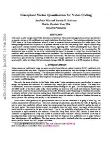
2.14 Results from Georgeson and Sullivan [?] showing equal-contrast contours for suprathreshold gratings of various spatial frequencies matched to 5 cpd gratings. . . . . . . . . . . . . . . . . . . . . . . . . . . . . .

29

iv

2.15 (A) Contrast matches between stimuli that vary in different dimensions of color space: luminance (lum), isoluminant red-green (LM), isoluminant blue-yellow (S), L-cone excitation only (L), and M-cone excitation only (M). The data show proportionality in contrast matches (solid lines). The dashed lines, slope equals 1, indicate the prediction for contrast based on equal cone contrast. (B) Average contrast-matching ratios across observers for the different pairwise comparisons of contrast. Diamonds indicate individual observers’ ratios. A ratio of 1 (dashed line) indicates prediction based on cone-contrast. From [?]. . . . . . . . . . .

30

2.16 Temporally counterphase modulated gratings change contrast over time sinusoidally producing a pattern that flickers. Each plot on the left shows the amplitude at a point in time. The luminance profile is simulated on the right. . . . . . . . . . . . . . . . . . . . . . . . . . . . . . . . . . .

33

2.17 (A) Temporal CSF as a function of mean luminance for a large flickering field. (B) The data in A are replotted in terms of amplitude rather than contrast. Replotted from [?]. . . . . . . . . . . . . . . . . . . . . . . .

34

2.18 (A) Spatial contrast sensitivity measured for gratings modulated at various temporal frequencies. (B) Temporal contrast sensitivity for gratings of various spatial frequencies. The mean luminance was held constant at 20 cd/m2 . From [?]. . . . . . . . . . . . . . . . . . . . . . . . . . .

35

2.19 A representation of a spatiotemporal contrast sensitivity surface. Redrawn from [?]. . . . . . . . . . . . . . . . . . . . . . . . . . . . . . .

36

v

List of Tables

vi

Chapter 2 Fundamentals of Human Vision and Vision Modeling Ethan D. Montag and Mark D. Fairchild Rochester Institute of Technology, Rochester, New York

2.1 Introduction Just as the visual system evolved to best adapt to the environment, video displays and video encoding technology is evolving to meet the requirements demanded by the visual system. If the goal of video display is to veridically reproduce the world as seen by the mind’s eye, we need to understand the way the visual system itself represents the world. This understanding involves finding the answer to questions such as: What characteristics of a scene are represented in the visual system? What are the limits of visual perception? What is the sensitivity of the visual system to spatial and temporal change? How does the visual system encode color information? In this chapter, the limits and characteristics of human vision will be introduced in order to elucidate a variety of the requirements needed for video display. Through an understanding of the fundamentals of vision, not only can the design principles for video encoding and display be determined but methods for their evaluation can be established. That is, not only can we determine what is essential to display and how to display it, but we can also decide on the appropriate methods to use to measure the quality of video display in terms relevant to human vision. In addition, an understanding of the

2.2. A Brief Overview of the Visual System

2

visual system can lead to insight into how rendering video imagery can be enhanced for aesthetic and scientific purposes.

2.2 A Brief Overview of the Visual System Our knowledge of how the visual system operates derives from many diverse fields ranging from anatomy and physiology to psychophysics and molecular genetics, to name a few. The physical interaction of light with matter, the electro-chemical nature of nerve conduction, and the psychology of perception all play a role. In his Treatise on Physiological Optics [vH11], Helmholtz divides the study of vision into three parts: 1) the theory of the path of light in the eye, 2) the theory of the sensations of the nervous mechanisms of vision, and 3) the theory of the interpretation of the visual sensations. Here we will briefly trace the visual pathway to summarize its parts and functions. Light first encounters the eye at the cornea, the main refractive surface of the eye. The light then enters the eye through the pupil, the hole in the center of the circular pigmented iris, which gives our eyes their characteristic color. The iris is bathed in aqueous humor, the watery fluid between the cornea and lens of the eye. The pupil diameter, which ranges from about 3 to 7 mm, changes based on the prevailing light level and other influences of the autonomic nervous system. The constriction and dilation of the pupil changes its area by a factor of 5, which as we will see later contributes little to the ability of the eye to adapt to the wide range of illumination it encounters. The light then passes through the lens of the eye, a transparent layered body that changes shape with accommodation to focus the image on the back of the eye. The main body of the eyeball contains the gelatinous vitreous humor maintaining the eye’s shape. Lining the back of the eye is the retina, where the light sensitive photoreceptors transduce the electromagnetic energy of light into the electro-chemical signals used by the nervous system. Behind the retina is the pigment epithelium that aids in trapping the light that is not absorbed by the photoreceptors and provides metabolic activities for the retina and photoreceptors. An inverted image of the visual field is projected onto the retina. The retina is considered an extension of the central nervous system and in fact develops as an outcropping of the neural tube during embryonic development. It consists of five main neural cell types organized into three cellular layers and two synaptic layers. The photoreceptors, specialized neurons that contain photopigments that absorb and initiate the neural response to light, are located on the outer part of the retina meaning that light must pass through all the other retinal layers before being detected. The signals from the photoreceptors are processed via the multitude of retinal connections and eventually exit the eye by way of the optic nerve, the axons of the ganglion cells, which make up the inner cellular layer of the retina. These axons are gathered together and exit the eye at the optic disc forming the optic nerve that projects to the lateral geniculate nucleus, a part of the thalamus in

2.2. A Brief Overview of the Visual System

3

the midbrain. From here, there are synaptic connections to neurons that project to the primary visual cortex located in the occipital lobe of the cerebral cortex. The human cortex contains many areas that respond to visual stimuli (covering 950 cm2 or 27% of the cortical surface [Ess03]) where processing of the various modes of vision such as form, location, motion, color, etc. occur. It is interesting to note that these various areas maintain a spatial mapping of the visual world even as the responses of neurons become more complex. There are two classes of photoreceptors, rods and cones. The rods are used for vision at very low light levels (scotopic) and do not normally contribute to color vision. The cones, which operate at higher light levels (photopic), mediate color vision and the seeing of fine spatial detail. There are three types of cones known as the short wavelength sensitive cones (S-cones), the middle wavelength sensitive cones (M-cones), and the long wavelength sensitive cones (L-cones), where the wavelength refers to the visible region of the spectrum between approximately 400 - 700 nm. Each cone type is colorblind; that is, the wavelength information of the light absorbed is lost. This is known as the Principle of Univariance so that the differential sensitivity to wavelength by the photoreceptors is due to the probability of photon absorption. Once a photopigment molecule absorbs a photon, the effect on vision is the same regardless of the wavelength of the photon. Color vision derives from the differential spectral sensitivities of the three cone types and the comparisons made between the signals generated in each cone type. Because there are only three cone types, it is possible to specify the color stimulus in terms of three numbers indicating the absorption of light by each of the three cone photoreceptors. This is the basis of trichromacy, the ability to match any color with a mixture of three suitably chosen primaries. As an indication of the processing in the retina, we can note that there are approximately 127 million receptors (120 million rods and 7 million cones) in the retina yet only 1 million ganglion cells in the optic nerve. This overall 127:1 convergence of information in the retina belies the complex visual processing in the retina. For scotopic vision there is convergence, or spatial summation, of 100 receptors to 1 ganglion cell to increase sensitivity at low light levels. However, in the rod-free fovea, cone receptors may have input to more than one ganglion cell. The locus of light adaptation is substantially retinal and the center-surround antagonistic receptive field properties of the ganglion cells, responsible for the chromatic-opponent processing of color and lateral inhibition, are due to lateral connections in the retina. Physiological analysis of the receptive field properties of neurons in the cortex has revealed a great deal of specialization and organization in their response in different regions of the cortex. Neurons in the primary visual cortex, for example, show responses that are tuned to stimuli of specific sizes and orientations (see [KNM84]). The area MT, located in the medial temporal region of the cortex in the macaque monkey, is area in which the cells are remarkably sensitive to motion stimuli [MM93]. Damage to homologous areas in humans (through stroke or accident, for example) has been thought to

4

2.3. Color Vision

cause defects in motion perception [Zek91]. Deficits in other modes of vision such as color perception, localization, visual recognition and identification, have been associated with particular areas or processing streams within the cortex.

2.3 Color Vision As pointed out by Newton, color is a property of the mind and not of objects in the world. Color results from the interaction of a light source, an object, and the visual system. Although the product of the spectral radiance of a source and the reflectance of an object (or the spectral distribution of an emissive source such as an LCD or a CRT display) specify the spectral power distribution of the distal stimulus to color vision, the color signal can be considered the product of this signal with the spectral sensitivity of the three cone receptor types. The color signal can therefore be summarized as 3 numbers that express the absorption of the three cone types at each “pixel” in the scene. Unfortunately, a standard for specifying cone signals has not yet been agreed upon, but the basic principles of color additivity have led to a description of the color signal that can be considered as linearly related to the cone signals.

2.3.1 Colorimetry Trichromacy leads to the principle that any color can be matched with a mixture of three suitable chosen primaries. We can characterize an additive match by using an equation such as: C1 = r1 R + g1 G + b1 B, (2.1) where the Red, Green, and Blue primaries are mixed together to match an arbitrary test light C by adjusting their intensities with the scalars r, g, and b. The amounts of each primary needed to make the match are known as the tristimulus values. The behavior of color matches follows the linear algebraic rules of additivity and proportionality (Grassmann’s laws) [WS82]. Therefore, given another match: C2 = r2 R + g2 G + b2 B,

(2.2)

the mixture of lights C1 and C2 can be matched by adding the constituent match components: C3 = C1 + C2 = (r1 + r2 )R + (g1 + g2 )G + (b1 + b2 )B. (2.3) Scaling the intensities of the lights retains the match (at photopic levels): kC3 = kC1 + kC2.

(2.4)

5

2.3. Color Vision

0.2

R

0. 4

0.8

C4

0.6

f t. o m A G

0.6

M

0. 8

0.4

C1

0.2

0.8

0.6

0.4

0.2

G

Amt. of R

B

A m t. B of

Figure 2.1: Maxwell diagram representing the concept of color-matching with three primaries, R, G, and B. The color match equations can therefore be scaled so that the coefficients of the primaries add to one representing normalized mixtures of the primaries creating unit amounts of the matched test light. These normalized weights are known as chromaticities and can be calculated by dividing the tristimulus value of each primary by the sum of all three tristimulus values. In this way matches can be represented in a trilinear coordinate system (a Maxwell diagram) as shown in Figure 2.1 [KB96]. Here a unit amount of C1 is matched as follows: C1 = 0.3R + 0.25G + 0.45B.

(2.5)

As shown in Equation (2.1) and Figure 2.1, the range of colors that can be produced by adding the primaries fill the area of the triangle bounded by unit amounts of the primaries. However if the primaries are allowed to be added to the test light, colors outside of this gamut can be produced, for example: C4 + bB = rR + gG = M,

(2.6)

6

2.3. Color Vision

where M is the color that appears in the matched fields. This can be rewritten as: C4 = rR + gG − bB,

(2.7)

where a negative amount of a primary means the primary is added to the test field. In Figure 2.1, an example is shown where: C4 = 0.6R + 0.6G − 0.2B.

(2.8)

Colorimetry is based on such color matching experiments in which matches to equal energy monochromatic test lights spanning the visible spectrum are made using real R, G, and B primaries. In this way, color can be specified based on the matching behavior of a standard, or average observer. One such case is the CIE 1931 (R,G,B) Primary System shown in Figure 2.2A in which monochromatic primaries of 700.0 (R), 536.1 (G), and 435.8 (B) were used to match equal-energy monochromatic lights along the visible spectrum in a 2◦ bipartite field. The color matching functions, r(λ), g(λ), and b(λ), shown in Figure 2.2A, represent the average tristimulus values of the matches. This system of matches was transformed to a set of matches made with imaginary primaries, X, Y, and Z, so that the color-matching functions, x(λ), y(λ), and z(λ), shown in Figure 2.2B, are all positive and the y(λ) color-matching function is the luminous efficiency function V (λ) to facilitate the calculation of luminance. As a result of additivity and proportionality, one can calculate the tristimulus values, X, Y , Z, for any color by integrating the product of the spectral power of the illuminant, the reflectance of the surface, and each of the color-matching functions: Z Z Z X = Sλ Rλ x(λ)dλ Y = Sλ Rλ y(λ)dλ Z = Sλ Rλ z(λ)dλ (2.9) λ

λ

λ

where Sλ is the spectral power distribution of the illuminant and Rλ is the spectral reflectance of the object. In practice, tabulated color-matching functions are used in summations to calculate the tristimulus values: X X X X=k Sλ Rλ x(λ)∆λ Y = k Sλ Rλ y(λ)∆λ Z = k Sλ Rλ z(λ)∆λ (2.10) λ

λ

λ

where k is a scaling factor used to define relative or absolute colorimetric values. Chromaticities can then be determined using: x = X/(X +Y +Z), y = Y /(X +Y +Z), and z = Z/(X + Y + Z) = 1 − x − y. The CIE 1931 (x,y) chromaticity diagram showing the spectral locus is shown in Figure 2.2C. Typically a color is specified by giving its (x,y) chromaticities and its luminance, Y . Ideally, the color-matching functions (the CIE has adopted two standard observers, the 1931 2◦ observer, above, and the 1964 10◦ observer based on color matches made using a larger field) can be considered a linear transform of the spectral sensitivities of

7

2.3. Color Vision

_ b

2

_ r

_ z

0.3

Tristimulus Values

1.5

700.0 nm

0.1

546.1 nm

0.2

435.8 nm

Tristimulus Values

_ g

_ x

0.5

0.0

−0.1

_ y 1

400

450

500

550

600

650

0

700

Wavelength, nm

400

450

500

550

600

650

700

Wavelength, nm 0.9 525

0.8 550

0.7 0.6

575

500

y

0.5 0.4

600 625 650 720

0.3 0.2 0.1

475 380

0 0

450

0.1

0.2

0.3

0.4

0.5

0.6

0.7

0.8

x

Figure 2.2: The CIE 1931 2◦ Standard Observer System of Colorimetry. A) (Top left) The color-matching functions based on real primaries R, G, and B. B) (Top right) The transformed color-matching functions for the imaginary primaries, X, Y,and Z. C) (Bottom) The (x, y) chromaticity diagram. the L-, M-, and S- cones. It is therefore possible to specify color in terms of L-, M- and S-cone excitation. Currently, work is underway to reconcile the data from color matching, luminous efficiency, and spectral sensitivity into a system that can be adopted universally. Until recently, specification of the cone spectral sensitivities has been a difficult problem because the overlap of their sensitivities makes it difficult to isolate these functions. A system of colorimetry based on L, M, and S primaries would allow a more direct and intuitive link between color specification and the early physiology of color vision [Boy96].

2.3. Color Vision

8

2.3.2 Color Appearance, Color Order Systems, and Color Difference A chromaticity diagram is useful for specifying color and determining the results of additive color mixing. However, it gives no insight into the appearance of colors. The appearance of a particular color depends on the viewer’s state of adaptation, both globally and locally, the size, configuration, and location of the stimulus in the visual field, the color and location of other objects in the scene, the color of the background and surround, and even the colors of objects presented after the one in question. Therefore, two colored patches with the same chromaticity and luminance may have wildly different appearances. Although color is typically thought of as being three-dimensional due to the trichromatic nature of color matching, five perceptual attributes are needed for a complete specification of color appearance [Fai98]. These are: brightness, the attribute according to which an area appears to be more or less intense; lightness, the brightness of an area relative to a similarly illuminated area that appears to be white; colorfulness (chromaticness), the attribute according to which an area appears to be more or less chromatic; chroma, the colorfulness of an area relative to a similarly illuminated area that appears to be white; and hue, the attribute of a color denoted by its name such as blue, green, yellow, orange, etc. One other common attribute, saturation, defined as the colorfulness of an area relative to its brightness, is redundant when these five attributes are specified. Brightness and colorfulness are considered sensations that indicate the absolute levels of the corresponding sensations while lightness and chroma indicate the relative levels of these sensations. In general, increasing the illumination increases the brightness and colorfulness of a stimulus while the lightness and chroma remain approximately constant. Therefore a video or photographic reproduction of a scene can maintain the relative attributes even though the absolute levels of illumination are not realizable. In terms of hue, it is observed that the colors red, green, yellow, and blue, are unique hues that do not have the appearance of being mixtures of other hues. In addition, they form opponent pairs so that perception of red and green cannot coexist in the same stimulus nor can yellow and blue. In addition, these terms are sufficient for describing the hue components of any unrelated color stimulus. This idea of opponent channels, first ascribed to Hering [Her64], indicates a higher level of visual processing concerned with the organization of color appearance. Color opponency is observed both physiologically and psychophysically in the chromatic channels with L- and M-cone (L-M) opponency and opponency between S-cones and the sum of the L- and M-cones (S-(L+M)). However, although these chromatic mechanisms are sure to be the initial substrate of red-green and yellow-blue opponency, they do not account for the phenomenology of Hering’s opponent hues. Even under standard viewing conditions of adaptation and stimulus presentation,

9

2.3. Color Vision

10RP

5R

White

10/

10R

1 2 3

5RP

4

5YR 6

7

9/

8 9

10P

8/

10YR

Bo un da ry of c

olo r

an tm

7/

5P

10Y

/2 /4 /6 /8

5PB

/10

Munsell value

10PB

ut m ga

5Y

ix tu re

6/ 5/

/2

/4

/6

/8

/10

4/

5GY 3/

10GY

10B 5G

5B

2/ 1/ Munsell chroma

10GB

5GB

10G

0/ Black

Figure 2.3: The organization of the Munsell Book of Colors. A) (Left) Arrangement of the hues in a plane of constant value. B) (Right) A hue leaf with variation in value and chroma. the appearances of colors represented in the CIE diagram do not represent colors in a uniform way that allows specification of colors in terms of appearance. Various color spaces have been developed as tools for communicating color, calculating perceptual color difference, and specifying the appearance of colors. The Munsell Book of Color [Nic76] is an example of a color-order system used for education, color communication, and color specification. The system consists of a denotation of colors and their physical instantiation arranged according to the attributes of value (lightness), chroma and hue. Figure 2.3A shows the arrangement of the hues in a plane of constant value in the Munsell Book of Color (R = red, YR = yellow-red, P = purple, etc.). Fig 2.3B shows a hue leaf with variation of value and chroma. The space is designed to produce a visually uniform sampling of perceptual color space when the samples are viewed under a standard set of conditions. The Munsell notation of a color is HV /C, where H represents hue, V represents value, and C represents chroma. The relationship between relative luminance (scaling Y of the white point to a value of 100) and the Munsell value, V , is the 5th -order polynomial: Y = 1.2219V − 0.23111V 2 + 0.23951V 3 − 0.021009V 4 + 0.0008404V 5

(2.11)

The CIE 1976 L∗ , a∗ , b∗ , (CIELAB), color space was adopted as an empirical uniform color space for calculating the perceived color difference between two col-

10

2.3. Color Vision

ors [CIE86]. The Cartesian coordinates, L∗ , a∗ , and b∗ , of a color correspond to a lightness dimension and two chromatic dimensions that are roughly red-green and blueyellow. The coordinates of color are calculated from its tristimulus values and the tristimulus values of a reference white so that the white is plotted at L∗ = 100, a∗ = 0, and b∗ = 0. The space is organized so that the polar transformations of the a∗ and b∗ ∗ coordinates give the chroma, Cab , and the hue angle, hab , of a color. The equations for calculating CIELAB coordinates are: L∗ a∗ b∗ ∗ Cab hab

= = = = =

116(Y /Yn )1/3 − 16 500[(X/Xn )1/3 − (Y /Yn )1/3 ] 200[(Y /Yn )1/3 − (Z/Zn)1/3 ] [a∗2 − b∗2 ]1/2 ∗ arctan( ab∗ )

(2.12)

where (X,Y ,Z) are the color’s CIE tristimulus values and (Xn , Yn , Zn ) are the tristimulus values of a reference white. For values of Y /Yn , X/Xn , and Z/Zn less than 0.01 the formulae are modified (see [WS82] for details). Lightness, L∗ , is an exponential function of luminance. There is also an “opponent-like” transform for calculating a∗ and b∗ . Figure 2.4 shows a typical CRT gamut plotted in CIELAB space. ∗ Color differences, ∆Eab , can be calculated using the CIELAB coordinates:

1/2 ∗ ∆Eab = (∆L∗ )2 + (∆a∗ )2 + (∆b∗ )2

(2.13)

∗ ∗ 2 ∗ 2 1/2 ∆Eab = (∆L∗ )2 + (∆Cab ) + (∆Hab )

(2.14)

∗ ∗ 2 ∗ 2 1/2 ∆Hab = (∆Eab ) − (∆L∗ )2 − (∆Cab )

(2.15)

Or in terms of the polar coordinates:

∗ where ∆Hab is defined as:

More recent research [LCR01] has led to modification of the CIELAB color difference equation to correct for observed nonuniformities in CIELAB space. A generic form of these advanced color difference equations [Ber00] is given as: 1 ∆E = kE

"

∆L∗ k L SL

2

+

∗ ∆Cab k C SC

2

+

∗ ∆Hab k H SH

2 #1/2

(2.16)

where kE , kL , kC , and kH are parametric factors that are adjusted according to differences in viewing conditions and sample characteristics and SL , SC , and SH are weighting functions for lightness, chroma and hue that depend on the position of the samples in CIELAB color space. It should be noted that the different color difference formu-

11

2.3. Color Vision

Figure 2.4: A CRT gamut plotted in CIELAB space. lae in the literature may have different magnitudes on average so that comparisons of performance based on ∆E values should be based on the relative rather than absolute values of the calculated color differences. Color appearance models [Fai98] attempt to assign values to the color attributes of a sample by taking into account the viewing conditions under which the sample is observed so that colors with corresponding appearance (but different tristimulus values) can be predicted. These models generally consist of a chromatic-adaptation transform that adjusts for the viewing conditions (e.g., illumination, white-point, background, and surround) and calculations of at least the relative color attributes. More complex models include predictors of brightness and colorfulness and may predict color appearance phenomena such as changes in colorfulness and contrast with luminance [Fai98]. Color spaces can then be constructed based on the coordinates of the attributes derived in the model. The CIECAM02 color appearance model [MFH+ 02] is an example of a color appearance model that predicts the relative and absolute color appearance attributes based on specifying the surround conditions (average, dim, or dark), the luminance of the adapting field, the tristimulus values of the reference white point, and the tristimulus values of the sample.

2.4. Luminance and the Perception of Light Intensity

12

2.4 Luminance and the Perception of Light Intensity Luminance is a term that has taken on different meanings in different contexts and therefore the concept of luminance, its definition, and its application can lead to confusion. Luminance is a photometric measure that has loosely been described as the “apparent intensity” of a stimulus but is actually defined as the effectiveness of lights of different wavelengths in specific photometric matching tasks [SS99]. The term is also used to label the achromatic channel of visual processing.

2.4.1 Luminance The CIE definition of luminance [WS82] is a quantity that is a constant times the integral of the product of radiance and V (λ), the photopic spectral luminous efficiency function. V (λ) is defined as the ratio of radiant flux at wavelength λm to that of wavelength λ, when the two fluxes produce the same luminous sensations under specified condition with a value of 1 at λm = 555 nm. Luminance efficiency is therefore tied to the tasks that are used to measure it. Luminance is expressed in units of candelas per square meter (cd/m2 ). To control for the amount of light falling on the retina, the troland (td) unit is defined as cd/m2 multiplied by the area of the pupil. The V (λ) function in use by the CIE was adopted by the CIE in 1924 and is based on a weighted assembly of the results of a variety of visual brightness matching and minimum flicker experiments. The goal of the V (λ) in the CIE system of photometry and colorimetry is to predict brightness matches so that given two spectral power distributions, P1λ and P2λ , the expression: Z Z P1λ V (λ)dλ = P2λ V (λ)dλ (2.17) λ

λ

predicts a brightness match and therefore additivity applies to brightness. In direct heterochromatic brightness matching, it has been shown that this additivity law, known as Abney’s law, fails substantially [WS82]. For example when a reference “white”, W, is matched in brightness to a “blue” stimulus, C1 , and to a “yellow” stimulus, C2 , the additive mixture of C1 and C2 is found to be less bright than 2W, a stimulus that is twice the radiance of the reference white [KB96]. Another example of the failure of V (λ) to predict brightness matches is known as the Helmholtz-Kohlrausch effect where chromatic stimuli of the same luminance as a reference white stimulus appear brighter than the reference. In Figure 2.5, we see the results from Sanders and Wyszecki [SW64] and presented in [WS82] that show how the ratio, B/L, of the luminance of a chromatic test color, B, to the luminance of a white reference, L, varies as a function of chroma and hue. Direct hetereochromatic brightness matching experiments


13

Figure 2.5: The Helmholtz-Kohlrausch effect in which the apparent brightness of isoluminant chromatic colors increases with chroma. The loci of constant ratios of the luminance of chromatic colors to a white reference (B/L) based on heterochromatic brightness matches of Sanders and Wyszecki [WS82, SW64] are shown in the CIE 1964 (x10 , y10 ) chromaticity diagram. From [WS82]. also demonstrate large inter-observer variability. Other psychophysical methods for determining “matches” have derived luminance efficiency functions that are more consistent between observers and obey additivity. Heterochromatic flicker photometry (HFP) is one such technique in which a standard light, λS , at a fixed intensity is flickered in alteration with a test light, λT , at a frequency of about 10 to 15 Hz [KB96]. The observer’s task is to adjust the intensity of λT to minimize the appearance of flicker in the alternating lights. The normalized reciprocal of the radiances of the test lights measured across the visible spectrum needed to minimize flicker is the resulting luminous efficiency function. Comparable results are obtained in the minimally distinct border method (MDB) in which the radiance of λT is adjusted to minimize the distinctness of the border between λT and λS when they are presented as precisely juxtaposed stimuli in a bipartite field [KB96]. Modifications of the CIE V (λ) function are aimed at achieving brightness additivity and proportionality by developing functions that are in better agreement to HFP and MDB data. The shape of the luminous efficiency function is often considered as the spectral sensitivity of photopic vision and as such it is a function of the sensitivity of the separate cone types. However, unlike the spectral sensitivities of the cones, the luminosity


14

function changes shape depending on the state of adaptation, especially chromatic adaptation [SS99]. Therefore the luminosity function only defines luminance for the conditions under which it was measured. As measured by HFP and MDB, the luminosity function can be modeled as a weighted sum of L- and M-cone spectral sensitivities with L-cones dominating. The S-cones contribution to luminosity is considered negligible under normal conditions. (The luminosity function of dichromats, those color-deficient observers who lack either the L- or M-cone photopigment, is the spectral sensitivity of the remaining longer wavelength sensitive receptor pigment. Protanopes, who lack the L-cone pigment, generally see “red” objects as being dark. Deuteranopes, who lack the M-cone pigment, see brightness similarly to color normal observers.)

2.4.2 Perceived Intensity As the intensity of a background field increases, the intensity required to detect a threshold increment superimposed on the background increases. Weber’s law states that the ratio of the increment to the background or adaptation level is a constant so that ∆I/I = k, where I is the background intensity and ∆I is the increment threshold (also known as the just noticeable difference or JND) above this background level. Weber’s law is a general rule of thumb that applies across different sensory systems. To the extent that Weber’s Law holds, it states that threshold contrast is constant at all levels of background adaptation so that a plot of ∆I versus I will have a constant slope. In vision research, plots of log(∆I) versus log(I), known as threshold versus intensity or t.v.i. curves, exhibit a slope of one when Weber’s law applies. The curve that results when the ratio, ∆I/I, the Weber fraction, is plotted against background intensity has a slope of zero when Weber’s law applies. The Weber fraction is a measure of contrast and it should be noted that contrast is a more important aspect of vision than the detection of absolute intensity. As the illumination on this page increases from dim illumination to full sunlight, the contrast of the ink to the paper remains constant even as the radiance of the reflected light off the ink in sunlight surpasses the radiance reflected off the white paper under dim illumination. If the increment threshold is considered a unit of sensation, one can build a scale of increasing sensation by integrating JNDs so that S = K log(I), where S is the sensation magnitude and K is a constant that depends on the particular stimulus conditions. The logarithmic relationship between stimulus intensity and the associated sensation is known as Fechner’s Law. The increase in perceptual magnitude is characterized by a compressive relationship with intensity as shown in Figure 2.6. Based on applicability of Weber’s law and the assumptions of Fechner’s Law, a scale of perceptual intensity can be constructed based on the measurement of increment thresholds using classical psychophysical techniques to determine the Weber fraction.


15

Weber’s law, in fact, does not hold for the full range of intensities that the visual system operates. However, at luminance levels above 100 cd/m2, typical of indoor lightning, Weber’s Law holds fairly well. The value of the Weber fraction depends upon the exact stimulus configuration with a value as low as 1% under optimal conditions [HF86]. In order to create a scale of sensation using Fechner’s Law, one would need to choose a Weber fraction that is representative of the conditions under which the scale would be used. Logarithmic functions have been used for determining lightness differences such as in the BFD color difference equation [LR87]. It should be noted, however, that ∆E values are typically larger than one JND. Since they do not represent true increment thresholds, Weber’s law may not apply. The validity of Fechner’s law has been questioned based on direct brightness scaling experiments using magnitude estimation techniques. Typically these experiments yield scales of brightness that are power functions of the form S = kI a , where S is the sensation magnitude, I is the stimulus intensity, a is exponent that depends on the stimulus conditions, and k is a scaling constant. This relationship is known as Stevens’ Power Law. For judgments of lightness, the exponent, a, typically has a value less than one demonstrating a compressive relationship between stimulus intensity and perceived magnitude. The value of the exponent is dependent on the stimulus conditions of the experiment used to measure it. Therefore, the choice of exponent must be based on data from experiments that are representative of the conditions in which the law will be applied. As shown above, the Munsell Book of Color, Equation (2.11), and the L∗ function in CIELAB, Equation (2.12) are both exponential functions. Figure 2.6 shows a comparison of various lightness vs luminance factor functions that are summarized in [WS82]. Functions based on Fechner’s Law (logarithmic functions) and power functions have been used for lightness scales, as shown in the figure. Although the mathematical basis of a lightness versus luminance factor function may be theoretically important, it is the compressive nonlinearity observed in the data that must be modeled. As seen in Figure 2.6, different functional relationships between luminance and lightness result depending on the exact stimulus conditions and psychophysical techniques used to collect the data. For example, curve 2 was observed with a white background, curves 1, 3, and 4 were obtained using neutral backgrounds with a luminance factor of approximately 20% (middle-gray), curve 6 was obtained on a background with a luminance factor of approximately 50%, and curve 5 was based on application of Fechner’s law applied to observations with backgrounds with luminance factors close to the gray chips being compared. The effect of the background influences the appearance of lightness in two ways.

16


10 9

V, lightness−scale value

8 7 6 5 4 3

2

3

4

1

1: Y = 1.2219V−0.23111V +0.23951V −0.021009V +0.0008404 2: V = Y 1/2 3: V = (1.474Y−0.00474Y 2) 1/2 4: V = 116 (Y/100) 1/3−16 5: V = 0.25+5 log Y 6: V = 6.1723 log (40.7Y/100+1)

0 0

20

2

40

60

80

5

100

Y, luminance factor

Figure 2.6: A variety of luminance versus lightness functions: 1) Munsell renotation system, observations on a middle-gray background; 2) Original Munsell system, observations on a white background; 3) Modified version of (1) for a middle-gray background; 4) CIE L∗ function, middle-gray background; 5) Gray scale of the Color Harmony Manual, background similar to the grays being compared; 6) Gray scale of the DIN Color Chart, gray background. Equations from [WS82]. Due to simultaneous contrast, a dark background will cause a patch to appear lighter while a light background will cause a patch to look darker. Sensitivity to contrast increases when the test patch is close to lightness of the background. Known as the crispening effect, this phenomenon leads to nonuniformities in the shapes of the luminance vs lightness function with different backgrounds and increased sensitivity to lightness differences when patches of similar lightness to the background are compared [WS82, Fai98]. In addition, the arrangement and spatial context of a pattern can influence the apparent lightness. White’s illusion [And03] is an example where a pattern of identical gray bars appears lighter (darker) when embedded in black (white) stripes although simultaneous contrast would predict the opposite effect due to the surrounding region. Figure 2.7 shows examples of simultaneous contrast, crispening, and White’s illusion.

2.5. Spatial Vision and Contrast Sensitivity

17

A

B

C

Figure 2.7: Various lightness illusions. A) Simultaneous contrast: The appearance of the identical gray squares changes due to the background. B) Crispening: The difference between the two gray squares is more perceptible when the background is close to the lightness of the squares. C) White’s illusion: The appearance of the identical gray bars changes when they are embedded in the white and black stripes.

2.5 Spatial Vision and Contrast Sensitivity Computational analysis has been the dominant paradigm for the study of visual processing of form information in the cortex replacing a more qualitative study based on identifying the functional specialization of cortical modularity and feature detection in cortical neurons. The response of the visual system to harmonic stimuli has been used to analyze the processing of the visual system to see whether the response to more complex stimuli can be modeled from the response of simpler stimuli in terms of linear systems analysis. Because the visual system is not a linear system, these methods reveal where more comprehensive study of the visual system is needed.

2.5.1 Acuity and Sampling The first two factors that need to be accounted for in the processing of spatial information by the visual system are the optics of the eye and the sampling of the visual scene by the photoreceptor array. Once the scene is sampled by the photoreceptor array, neural


18

processing determines the visual response to spatial variation. Attempts to measure the modulation transfer function (MTF) of the eye have relied on both physical and psychophysical techniques. Campbell and Gubisch [CG66], for example, measured the linespread function of the eye by measuring the light from a bright line stimulus reflected out of the eye and correcting for the double passage of light through the eye for different pupil sizes. MTFs derived from double-pass measurements correspond well with psychophysical measurements derived from laser interferometry in which the MTF is estimated from the ratio of contrast sensitivity to conventional gratings and interference fringes that are not blurred by the optics of the eye [WBMN94]. The MTF of the eye demonstrates that for 2 mm pupils, the modulation of the signal falls off very rapidly and is approximately 1% at about 60 cpd. For larger pupils, 4-6 mm, the modulation falls to 1% at approximately 120 cpd [PW03]. In the fovea the cone photoreceptors are packed tightly in a triangular arrangement with a mean center-to-center spacing of 32 arc min [Wil88]. This corresponds to a sampling rate of approximately 120 samples per degree or a Nyquist frequency of around 60 cpd. Because the optics of the eye sufficiently degrade the image above 60 cpd we are spared the effects of spatial aliasing in normal foveal vision. The S-cone packing in the retina is much more sparse than the M- and L-cone packing so that its Nyquist limit is approximately 10 cpd [PW03]. Visual spatial acuity is therefore considered to be approximately 60 cpd although under special conditions, for example, peripheral vision, large pupil sizes, and laser interferometry, higher spatial frequencies can be either directly resolved or seen via the effects of aliasing. This would appear to set a useful limit for the design of displays, for example. However, in addition to the ability of the visual system to detect spatial variation, there also exists the ability to detect spatial alignment known as Vernier acuity or hyperacuity. In these tasks, observers are able to judge whether two stimuli (dots or line segments) separated by a small gap are misaligned with offsets as small as 2-5 arc sec, which is less than one-fifth the width of a cone [WM77]. It is hypothesized that it is the blurring of the optics of eye that contributes to this effect by distributing the light over a number of receptors. By comparing the distributions of the responses to the two stimuli, the visual system can localize the position of the stimuli at a resolution finer than the receptor spacing [Wan95, DD90].

2.5.2 Contrast Sensitivity It can be argued that the visual system evolved to discriminate and identify objects in the world. The requirements for this task are different from those needed if the purpose of the visual system was meant to measure and to record the variation of light intensity in the visual field. In this regard, characterization of the visual system’s response to variations in contrast as a function of spatial frequency is studied using harmonic stimuli.

19


2

1000 cd/m

100 cd/m2

Contrast sensitivity

100

2

10 cd/m 2

1 cd/m

10

2

0.1 cd/m

2

0.01 cd/m

1 0.1

1

10

100

Spatial frequency (cycles/degree)

Figure 2.8: Contrast sensitivity function for different mean luminance levels. The curves were generated using the empirical model of the achromatic CSF in [Bar04]. The contrast sensitivity function (CSF) plots the sensitivity of the visual system to sinusoids of varying spatial frequency. Figure 2.8 shows the contrast sensitivity of the visual system based on Barten’s empirical model [Bar99, Bar04]. The contrast sensitivity is a plot of the reciprocal of the threshold (ordinate) contrast needed to detect sinusoidal gratings of different spatial frequency (abscissa) in cycles per degree of visual angle. Contrast is usually given using Michelson contrast: (Lmax − Lmin )/(Lmax + Lmin ), where Lmax and Lmin are the peak and trough luminance of the grating, respectively. Typically plotted on log-log coordinates, the CSF reveals the limits of detecting variation in intensity as a function of size. Each curve in Figure 2.8 shows the change in contrast sensitivity for sinusoidal gratings modulated around mean luminance levels ranging from 0.01 cd/m2 to 1000 cd/m2 . As the mean luminance increases to photopic levels the CSF takes on its characteristic band-pass shape. As luminance increases, the high frequency cut-off, indicating spatial acuity, increases. At scotopic light levels, reduced acuity is due to the increased spatial pooling in the rod pathway which increases absolute sensitivity to light. As the mean luminance level increases the contrast sensitivity to lower spatial frequencies increases and then remains constant. Where these curves converge and overlap, we see that the threshold contrast is constant despite the change in mean luminance. This is where Weber’s law holds. At higher spatial frequencies, Weber’s Law breaks down. The exact shape of the CSF depends on many parametric factors so that there is no


20

one canonical CSF curve [Gra89]. Mean luminance, spatial position on the retina, spatial extent (size), orientation, temporal frequency, individual differences, and pathology are all factors that influence the CSF. (See [Gra89] for a detailed bibliography of studies related to parametric differences.) Sensitivity is greatest at the fovea and tends to fall off linearly (in terms of log sensitivity) with distance from the fovea for each spatial frequency. This fall off is faster for higher spatial frequencies so that the CSF becomes more low-pass in the peripheral retina. As the spatial extent (the number of periods) in the stimulus increases, there is an increase in sensitivity up to a point at which sensitivity remains constant. The change in sensitivity with spatial extent changes as the distance from the fovea increases so that the most effective stimuli in the periphery are larger than in the fovea. The oblique effect is the term applied to the reduction in contrast sensitivity to obliquely oriented gratings compared to horizontally and vertically ones. This reduction in sensitivity (a factor of 2 or 3) occurs at high spatial frequencies.

2.5.3 Multiple Spatial Frequency Channels Psychophysical, physiological, and anatomical evidence suggest that the CSF represents the envelope of the sensitivity of many more narrowly tuned channels as shown in Figure 2.9. The idea is that the visual system analyzes the visual scene in terms of multiple channels each sensitive to a narrow range of spatial frequencies. In addition to channels sensitive to narrow bands of spatial frequency, the scene is also decomposed into channels sensitive to narrow bands of orientation. This concept of multiresolution representations forms the basis of many models of spatial vision and pattern sensitivity (see [Wan95, DD90]). The receptive fields of neurons in the visual cortex are size specific and therefore show tuning functions that correspond with multiresolution theory and may be the physiological underpinnings of the psychophysical phenomena described below. Physiological evidence points to a continuous distribution of peak frequencies in cortical cells [DD90] although multiresolution models have been built using a discrete number of spatial channels and orientations (e.g., Wilson and Regan [WR84] suggested a model with six spatial channels at eight orientations). Studies have shown that six channels seem to model psychophysical data well without ruling out a larger number [WLM+ 90]. Both physiological and psychophysical evidence indicate that the bandwidths of the underlying channels are broader for lower frequency channels and become narrower at higher frequencies as plotted on a logarithmic scale of spatial frequency. On a linear scale, however, the low-frequency channels have a much narrower bandwidth than the high-frequency channels.

21

Log Contrast Sensitivity


Log Spatial Frequency Figure 2.9: The contrast sensitivity function represented as the envelope of multiple, more narrowly tuned spatial frequency channels. 2.5.3.1 Pattern adaptation Figure 2.10A is a demonstration of the phenomenon of pattern adaptation first described by Pantle and Sekuler [PS68] and Blakemore and Campbell [BC69]. The two patterns in the center of Figure 2.10A, the test patterns, are of the same spatial frequency. The adaptation patterns on the left are higher (top) and lower (bottom) spatial frequencies. By staring at the fixation bar between the two adaptation patterns for a minute or so, the channels that are tuned to those spatial frequencies adapt, or become fatigued, so that their response is suppressed for a short period of time subsequent to adaptation. After adaptation, the appearance of the two test patterns is no longer equal. The top pattern now appears to be of a higher spatial frequency and the bottom appears lower. The response of the visual system depends on the distribution of responses in the spatial channels. Before adaptation, the peak of the response is located in the channels tuned most closely to the test stimulus. Adaptation causes the channels most sensitive to the adaptation stimuli to respond less vigorously. Upon subsequent presentation of the test pattern, the distribution of response is now skewed from its normal distribution so that higher-frequency adaptation pattern will lead to relatively more response in the lower-frequency channels and vice versa. Measurement of the CSF after contrast adaptation reveals a loss of sensitivity in the region surrounding the adaptation frequency as shown in Figure 2.10B. This effect of adaptation has been shown to be independent of phase [JT75] demonstrating that phase information is not preserved in pattern adapta-


22

A

Log Contrast Sensitivity

B

Log Spatial Frequency

Figure 2.10: Pattern and orientation adaptation. A) After adapting to the two patterns on the left by staring at the fixation bar in the center for a minute or so, the two identical patterns in the center will appear to have different widths. Similarly, adaptation to the tilted patterns on the right will cause an apparent orientation change in the central test patterns. B) Adaptation to a specific spatial frequency (arrow) causes a transient loss in contrast sensitivity in the region of the adapting frequency and a dip in the CSF. tion. Adaptation to the two right hand patterns in Figure 2.10A leads to a change in the apparent orientation of the test patterns in the center. As with spatial frequency, the response of the visual system to orientation depends on the pattern of response in multiple channels tuned to different orientations. Adaptation to a particular orientation will fatigue those channels that are more closely tuned to that particular orientation so that the pattern of response to subsequent stimuli will be skewed [BC69]. 2.5.3.2 Pattern detection Campbell and Robson [CR68] measured the contrast detection thresholds for sine wave gratings and a variety of periodic complex waveforms (such as square waves and sawtooth gratings) and found that the detection of complex patterns were determined by the


23

contrast of the fundamental component rather than the contrast of the overall pattern. In addition, they observed that the ability to distinguish a square wave pattern from a sinusoid occurred when the third harmonic of the square wave reached its own threshold contrast. Graham and Nachmias [GN71] measured the detection thresholds for gratings composed of two frequency components, f and 3f , as a function of the relative phase of the two gratings. When these two components are added in phase so that their peaks coincide, the overall contrast is higher than when they are combined so that their peaks subtract. However, the thresholds for detecting the gratings were the same regardless of phase. These results support a spatial frequency analysis of the visual stimulus as opposed to detection based on the luminance profile. 2.5.3.3 Masking and facilitation The experiments on pattern adaptation and detection dealt with the detection and interaction of gratings at their contrast threshold levels. The effect of suprathreshold patterns on grating detection is more complicated. In these cases a superimposed grating can either hinder the detection (masking) of a test grating or it can lead to a lower detection threshold (facilitation), depending on the properties of the two gratings. The influence of the mask on the detectability of the test depends on the spatial frequency, orientation, and phase of the mask relative to the test. This interaction increases as the mask and target become more similar. For similar tests and masks, facilitation is seen at low mask contrasts and as the contrast increases the test is masked. In the typical experimental paradigm a grating (or a Gabor pattern) of a fixed contrast called the “pedestal” or “masking grating” is presented along with a “test” or “signal” grating (or Gabor). The threshold contrast at which the test can be detected (or discriminated in a forced-choice) is measured as a function of the contrast of the mask. The resulting plot of contrast threshold versus the masking contrast is sometimes referred to as the threshold versus contrast, or TvC, function. Figure 2.11 shows the results from Legge and Foley [LF80]. In these experiments both the mask and test were at the same orientation. As the spatial frequency of the mask approaches the same frequency of the test we see facilitation at low contrasts. At higher mask contrasts the detection of the target is masked leading to an elevation in the contrast threshold. The initial decrease and subsequent increase seen in these curves is known as the “dipper effect”. In Figure 2.11, we see that this masking is slightly diminished when the mask frequency is much different from that of the test. Other studies (e.g., [SD83, WMP83]) have shown that the effectiveness of the masking is reduced as the mask and test frequencies diverge showing a characteristic band-limited tuning response. These masking effects support the multiresolution theory.


24

Figure 2.11: Contrast masking experiment showing masking and facilitation by the masking stimulus. The threshold contrasts (ordinate) for detecting a 2 cpd target grating are plotted as a function of the contrast of a superimposed masking grating. Each curve represents the results for a mask of a different spatial frequency. Mask frequencies ranged from 1 to 4 cpd. The curves are displaced vertically for clarity. The dashed lines indicate the unmasked contrast threshold. From [LF80]. There is no effect of the phase relationship between the mask and test at higher masking contrasts where masking is observed. However, the relative phase of the mask and test are critical at low mask contrasts where facilitation is seen [BW94, FC99]. Foley and Chen [FC99] describe a model of contrast discrimination that explains both masking and facilitation and the dependence of phase on facilitation in which spatial phase is an explicit parameter of the model. Yang and Makous’ [YM95] model of contrast discrimination models the phase relationship seen in the dipper effect without specific phase parameters. Bowen and Wilson [BW94] attribute the dipper effect to local adaptation preceding spatial filtering. Both adaptation and masking experiments have been used to determine the bandwidths of the underlying spatial frequency channels. The estimates of bandwidth, al-


25

though variable, correspond to the bandwidths of cells in the primary visual cortex of animals studied using physiological techniques [DD90, WLM+ 90]. Experiments studying the effect of orientation of the mask on target detection have shown that as the orientation of the mask approaches that of the target, the threshold contrast for detecting the target increases. Phillips and Wilson [PW84], for example, measured the threshold elevation caused by masking for various spatial frequencies and masking contrasts. Their estimates of the orientation bandwidths show a gradual decrease in bandwidth of about ±30◦ at 0.5 cpd to ±15◦ at 11.3 cpd which agrees well with physiological results from macaque striate cortex. No differences were found for tests oriented at 0◦ and 45◦ indicating that the oblique effect is not due to differences in bandwidth at these two orientations but rather is more likely due to a predominance of cells with orientation specificity to the horizontal and vertical [PW84]. The same relationships found between the spatial and orientation tuning of visual mechanism elucidated using the psychophysical masking paradigm agree with those revealed in recordings from cells in the macaque primary cortex [WLM+ 90]. 2.5.3.4 Nonindependence in spatial frequency and orientation The multiresolution representation theory postulates independence among the various spatial frequency and orientation channels that are analyzing the visual scene. Models of spatial contrast discrimination are typically based on the analysis of the stimulus through independent spatial frequency channels followed by a decision stage in which the outputs from these channels are compared (e.g., [FC99, WR84]). However, there is considerable evidence of nonlinear interactions between separate spatial frequency and orientation channels that challenge a strong form of the multiresolution theory (see [Wan95]). Both physiologically and psychophysically, there is evidence of interactions between channels that are far apart in their tuning characteristics. Figure 2.12 shows two perceptual illustrations of nonlinear interaction for spatial frequency (Figure 2.12A) and orientation (Figure 2.12B). Figure 2.12A shows a grating of frequency f , top, and a grating that is the sum of gratings of 4f , 5f , and 6f . The appearance of the complex grating has a periodicity of frequency f although there is no component at this frequency. Even though the early cortical mechanisms tuned to f are not responding to the complex grating, the higher frequency mechanisms tuned to the region of 5f somehow produce signals that fill in the “missing fundamental” during later visual processing (see [DD90]). Figure 2.12B shows the grating produced by the sum of two gratings at ±67.5◦ from the vertical. Although there is no grating components in the horizontal or vertical direction, there is the appearance of such stripes. Derrington and Henning [DH89] performed a masking experiment in which individual grating at orientations of ±67.5◦ did not mask


26

Figure 2.12: (A) The top grating has a spatial frequency of f . A perceived periodicity of f is seen in the complex grating on the bottom that is the sum of the frequencies of 4f , 5f , and 6f . Redrawn from [DD90]. (B) The sum of two gratings at ±67.5◦ has no horizontal or vertical components yet these orientations are perceived. the detection of a vertical grating of the same spatial frequency but the mixture of the two gratings produced substantial masking. De Valois [DD90] presents further examples of interactions between spatial frequency channels from adaptation experiments, physiological recordings, and anatomical studies in animals. These studies point to mutual inhibition among spatial frequency and orientation selective channels. 2.5.3.5 Chromatic contrast sensitivity Sensitivity to spatial variation for color has also been studied using harmonic stimuli. Mullen [Mul85] measured contrast sensitivity to red-green and blue-yellow gratings using counterphase monochromatic stimuli for the chromatic stimuli. The optics of the eye produce chromatic aberrations and magnification differences between the chromatic gratings. These artifacts were controlled by introducing lenses to independently focus each grating and scaling the size of the gratings. In addition, the relative luminances of the gratings were matched at the different spatial frequencies using flicker photometry.


27

Figure 2.13: Contrast sensitivity functions of the achromatic luminance channel and the red-green, and blue yellow opponent chromatic channels from [Mul85]. Solid lines indicate data from one subject. Dashed lines are extrapolated from the measured data to show the high-frequency acuity limit for the three channels in this experiment. Redrawn from Mullen [Mul85]. The wavelengths for the chromatic gratings were chosen to isolate the two chromaticopponent mechanisms. Figure 2.13 shows the resulting luminance and isolumant red-green and blue-yellow CSFs redrawn from one observer in Mullen. The chromatic CSFs are characterized by a low-pass shape and have high frequency cut-offs at much lower spatial frequencies than the luminance CSF. The acuity of the blue-yellow mechanism is limited by the sparse distribution of S-cones in the retinal mosaic, however the lower acuity in the red-green mechanism is not limited by retinal sampling and is therefore imposed by subsequent neural processing [Mul85, SWB93b]. Sekiguchi et al. [SWB93b, SWB93a] used laser interferometry to eliminate chromatic aberration with drifting chromatic gratings moving in opposite directions to simultaneously measure the chromatic and achromatic CSFs. They found a close match between the two chromatic mechanisms and slightly higher sensitivity than Mullens’s results. Poirson and Wandell [PW95] used an asymmetric color-matching task to explore the relationship between pattern vision (spatial frequency) and color appearance. In this task, square-wave gratings of various spatial frequencies composed of pairs of complementary colors (colors whose additive mixture is neutral in appearance) were presented to observers. The observers’ task was to match the color of a 2-degree square patch to the colors of the individual bars of the square-wave grating. They found that the color appearance of the bars depended on the spatial frequency of the pattern. Using a pattern-


28

color separable model, Poirson and Wandell derived the spectral sensitivities and spatial contrast sensitivities of the three mechanisms that mediated the color appearance judgments. These mechanisms showed a striking resemblance to the luminance and two chromatic-opponent channels identified psychophysically and physiologically. One outcome of the difference in the spatial response between the chromatic and luminance channels is that the sharpness of an image is judged based on the sharpness of the luminance information in the image since the visual system is incapable of resolving high-frequency chromatic information. This has been taken advantage of in the compression and transmission of color images since the high spatial frequency chromatic information in an image can be removed without a loss in perceived image quality (e.g., [MF85]). The perceptual salience of many geometric visual illusions is severely diminished or eliminated when they are reproduced using isoluminant patterns due to this loss of high spatial frequency information. The minimally distinct border method for determining luminance matches is also related to the reduced spatial accuity of the chromatic mechanisms. 2.5.3.6 Suprathreshold contrast sensitivity The discussion so far has focused on threshold measurements of contrast. Our sensitivity to contrast at threshold is very dependent on spatial frequency and has been studied in-depth to understand the limits of visual perception. The relationship between the perception of contrast and spatial frequency at levels above threshold will be briefly discussed here. It should be noted that there is increasing evidence that the effects seen at threshold are qualitatively different from those at suprathreshold levels so that models of detection and discrimination may not be applicable (e.g., [FBM03]). Figure 2.14 presents data for one subject redrawn from Georgeson and Sullivan [GS75] showing the results from a suprathreshold contrast matching experiment. In this experiment observers made apparent contrast matches between a standard 5 cpd grating and test gratings that varied from 0.25 to 25 cpd. The uppermost contour reflects the CSF at threshold. As the contrast of the gratings increased above threshold levels, the results showed that the apparent contrast matched when the physical contrasts were equal. This flattening of the equal-contrast contours in Figure 2.14 is more rapid at higher spatial frequencies. The flattening of the contours was termed “contrast constancy”. Subjects also made contrast matches using single lines and band-pass filtered images. Again it was shown that the apparent contrast matched the physical contrast when the stimuli were above threshold. Further experiments demonstrated that these results were largely independent of mean luminance level and position on the retina. Georgeson and Sullivan suggest that an active process is correcting the neural and optical blurring seen at threshold for high spatial frequencies. They hypothesize that the various spatial frequency channels adjust their gain independently in order to achieve

29


0.003

Contrast

0.01 0.03 0.1 0.3 1.0

0.25

0.5

1

2

5

5

10

15 20 25

Spatial frequency (c/deg)

Figure 2.14: Results from Georgeson and Sullivan [GS75] showing equal-contrast contours for suprathreshold gratings of various spatial frequencies matched to 5 cpd gratings. contrast constancy above threshold. This process, they suggest, is analogous to deblurring techniques used to compensate for the modulation transfer function in photography. Vimal [Vim00] found a similar flattening effect and chromatic contrast constancy for isoluminant chromatic gratings, however he proposed that different mechanisms underlie this process. Switkes and Crognale [SC99] compared the apparent contrast of gratings that varied in color and luminance in order to gauge the relative magnitude of contrast perception and the change of contrast perception with increasing contrast. In these experiments, contrast was varied in 1 cpd gratings modulated in five different directions in color space: luminance (lum), isoluminant red-green (LM), isoluminant blue-yellow (S), Lcone excitation only (L), and M-cone excitation only (M). A threshold procedure was used to determine equivalent perceptual contrast matches between pairs of these gratings at various contrast levels. The results are shown in Figure 2.15. Contrast was measured in terms of cone contrast, which is the deviation in cone excitation from the mean level. Although the authors considered that the cross-modal matching (color against luminance) task might be difficult due to the problem of comparing “apples vs. oranges” they found very good inter- and intra- observer consistency. The results of the experiment showed that the contrast matches between pairs of stimuli that varied in the different dimensions were proportional so that a single scaling factor could be used to describe the contrast matches between the stimuli as they varied in physical contrast. In Figure 2.15A, the matches between luminance and blue-yellow (top), red-green and blueyellow (middle), and L-cone and M-cone (bottom) gratings are shown for increasing levels of contrast. Matches are determined symmetrically so that error bars are determined in both dimensions. Looking at the top panel of Figure 2.15A, we see that as the physical contrast of the luminance grating and the blue-yellow grating increases, the


30

Figure 2.15: (A) Contrast matches between stimuli that vary in different dimensions of color space: luminance (lum), isoluminant red-green (LM), isoluminant blue-yellow (S), L-cone excitation only (L), and M-cone excitation only (M). The data show proportionality in contrast matches (solid lines). The dashed lines, slope equals 1, indicate the prediction for contrast based on equal cone contrast. (B) Average contrast-matching ratios across observers for the different pairwise comparisons of contrast. Diamonds indicate individual observers’ ratios. A ratio of 1 (dashed line) indicates prediction based on cone-contrast. From [SC99]. perceived contrast match is always at the same ratio of physical contrast (a straight line can be fit to the data). Much more S-cone contrast is needed to match the L- and Mcone contrast in the luminance grating. Figure 2.15B summarizes the results of the experiment by showing the ratio of conecontrasts needed to produce contrast matches for the different pairs of color and luminance contrasts. For example, for the data in the top panel of Figure 2.15A, the slope of the line fit to the data corresponds to the matching ratio labeled S/lum. These results indicate the physical scaling needed to match luminance and chromatic gratings at least at the spatial frequency tested. These data shed light on the performance of the visual system along different axes in color space by providing a metric for scaling the salience of these mechanisms [SC99].


31

2.5.3.7 Image compression and image difference Despite the fact that studies of the ability of the human visual system to detect and discriminate patterns do not give a complete understanding of how the visual system works to produce our final representation of the world, this information on perceptual limits can have practical use in imaging applications. For image compression, we can use this information to help guide the development of perceptually lossless encoding schemes. Similarly, we can use this information to eliminate information from imagery to which the visual system is insensitive in order to compute image differences based on what is visible in the scene. In his book, Foundations of Vision, Wandell [Wan95] introduces the concepts of the discrete cosine transformation in JPEG image compression, image compression using Laplacian pyramids, and wavelet compression. He points out the similarities between these algorithms and the multiresolution representation theory of pattern vision. Perceptually lossless image compression is possible because of the ability to quantize high spatial frequency information in the transformed image. Glenn [Gle93] enumerates and quantifies how the visual effects based on thresholds, which have been described in part here, such as the luminance and chromatic CSFs, pattern masking, the oblique effect, and temporal sensitivity (see below) can contribute to perceptually lossless compression. Zeng et al. [ZDL02] summarize the “visual optimization tools” based on spatial frequency sensitivity, color sensitivity, and visual masking that are used in JPEG 2000 in order to optimize perceptually lossless compression. It was pointed out above that the reduced resolution of the chromatic channels had been taken advantage of in image compression and transmission. This difference in the processing of chromatic and achromatic vision has been used for describing image differences in Zhang and Wandell’s extension of CIELAB for digital image reproduction called S-CIELAB for Spatial-CIELAB (Zhang and Wandell [ZW96, ZW88]). This method is intended to compute the visible color difference for determining errors in color image reproduction. In this procedure, an original color image and a reproduction are each converted into three bands corresponding to the luminance and two opponent chromatic channels. From here, each band is convolved with a spatial filter that removes the information beyond the limits of contrast visibility. The images are then converted into CIELAB coordinates where pixel-by-pixel color differences can be computed. Johnson and Fairchild [JF02, JF03] explored the use of different CSF functions, including the standard S-CIELAB filters, on their ability to predict image differences. They found that the use of filters that were normalized to maintain the DC component of the image performed better [JF02]. This also has an effect of boosting the gain for certain spatial frequencies since the function produces a filter with coefficients greater than one when the DC component is fixed at a value of one. In addition, they found that

2.6. Temporal Vision and Motion

32

anisotropic filters (with parameters that predict the oblique effect), such as the one used in Daly’s Visible Difference Predictor [Dal93], improve the predictions of the image difference model. Johnson and Fairchild [JF02] also applied spatial frequency adaptation, both a generic statistical model based on the 1/f approximation of spatial frequency content in natural scenes and an image dependent model, in their image difference predictor and found improvement. This adaptation tends to shift the peak of the CSF to higher frequencies.

2.6 Temporal Vision and Motion The sensitivity of the visual system to change over time and the perception of object motion are often linked together because the stimuli for motion produce temporal variations in light intensity falling on the retina. It follows that the perception of motion, at the early stages of visual processing, is driven by the same mechanisms that detect changes in intensity over time. In this section, the response of the visual system to temporally periodic stimuli will be briefly presented, followed by a short discussion of real and apparent motion.

2.6.1 Temporal CSF Before the application of linear systems theory to the study of temporal vision, the literature was dominated by studies that examined the temporal sensitivity of the eye in terms of the critical flicker frequency (CFF) of periodic waveforms modulated in amplitude [Wat86]. CFF refers to the temporal frequency (Hz) at which the perception of flicker in the stimulus changes to a steady or fused appearance. Two concepts that emerged from this work are the Ferry-Porter law and the Talbot-Plateau law. The FerryPorter law states that CFF rises linearly with the logarithm of the time-average background intensity. The Talbot-Plateau law states that the perceived intensity of a fused periodic stimulus is the same as a steady stimulus of the same time-average intensity. De Lange [de 54, de 58] introduced the ability to modulate temporal contrast while keeping the time-average background constant, which allowed the measurement of CFF and temporal contrast sensitivity at various mean intensities and temporal frequencies. His application of linear systems theory produced a coherent framework for interpreting the literature on temporal sensitivity [Wat86]. In a typical experiment for the measurement of temporal contrast sensitivity a grating is modulated temporally in counterphase so that the contrast reverses sinusoidally over time (see Figure 2.16). The contrast threshold for detecting a pattern is measured as a function of both the temporal frequency of the modulation and the spatial frequency of

33


Time

the pattern.

Space Figure 2.16: Temporally counterphase modulated gratings change contrast over time sinusoidally producing a pattern that flickers. Each plot on the left shows the amplitude at a point in time. The luminance profile is simulated on the right. Figure 2.17A shows the results from Kelly [Kel61] of the temporal contrast sensitivity of a large 68◦ field presented for frequencies from 1.6 to 75 Hz and mean luminances ranging from 0.06 to 9300 trolands. For these low spatial frequency stimuli, the shape of the temporal CSF is bandpass with a peak sensitivity at approximately 20 Hz at the highest luminance levels. As the mean luminance level decreases, curves become more low pass as the peak sensitivity decreases and shifts to lower frequencies. The overlapping sections of the curves for the moderate to high luminance levels indicate the region where Weber’s law holds. The CFF shifts to higher frequencies with increased luminance. In Figure 2.17B the data are replotted so that the reciprocal of threshold amplitude, rather than contrast, is plotted on the ordinate. When plotted in this manner, the high frequency portions of the curves at all luminance levels converge. This convergence indicates that at high flicker rates, the visual system cannot adapt to the signal and the response is linear. Robson [Rob66] first explored the relationship between spatial and temporal contrast sensitivity using temporally modulated counterphase gratings (see Figure 2.16) at a variety of spatial and temporal frequencies. The results of this experiment are shown in Figure 4.18. Here the mean luminance was 20 cd/m2 . The data are presented two ways. Figure 2.18A shows the spatial CSFs for gratings flickered from 1 to 22 Hz. We see that as the temporal frequency increases the spatial CSF changes from band-pass to low-pass. This indicates that the process responsible for the low spatial frequency atten-

34


200

A

B 100

100 10

1/Amplitude

Contrast Sensitivity

50

20

10

1.0

.1

5

2

1

.01

9300 td 850 td 77 td 7.1 td 0.65 td 0.06 td

2

5

.001 10

20

Frequency (Hz)

50

2

5

10

20

50

Frequency (Hz)

Figure 2.17: (A) Temporal CSF as a function of mean luminance for a large flickering field. (B) The data in A are replotted in terms of amplitude rather than contrast. Replotted from [Kel61]. uation is time dependent. Figure 4.18B shows the temporal CSFs for gratings varying in spatial frequency from 0.5 to 22 cpd. Here we see that the temporal CSF is bandpass at low spatial frequencies. We can infer here that the mechanism responsible for suppressing temporal contrast sensitivity is size dependent. It is remarkable to note the similarities between the spatial and temporal mechanism seen in Figure 2.18. Families of curves such as those in Figure 2.18 can be accumulated to produce a spatiotemporal contrast-sensitivity contour for a given mean luminance level. Here contrast sensitivity is plotted as a function of both temporal and spatial frequency. Figure 2.19 is a characterization of this surface [BK80]. Similar results are obtained with drifting gratings moving at various velocities. The spatiotemporal contrast response to chromatic stimuli has also been measured (see [Kel83, Kel89]). The response of the visual system to isoluminant red-green gratings exhibits much less attenuation at low temporal and spatial frequencies so that the shape of the spatiotemporal contrast surface is much more low-pass, especially above 0.5 Hz. The CFFs of the chromatic mechanisms occur at a lower temporal frequency than that of the achromatic channel.


35

Figure 2.18: (A) Spatial contrast sensitivity measured for gratings modulated at various temporal frequencies. (B) Temporal contrast sensitivity for gratings of various spatial frequencies. The mean luminance was held constant at 20 cd/m2 . From [Rob66].

2.6.2 Apparent Motion There are a number of ways in which the appearance of motion occurs without any real movement in the stimulus. For example, adaptation to motion in a particular direction will lead to a motion aftereffect in the opposite direction. The moon can appear to move behind the clouds due to induced motion because of a misjudged frame of reference. Apparent motion, or stroboscopic motion, is the most common case of perceived motion without a real moving stimulus. Consider an object at position 1 at time 1. At some point in time, time 2, the object disappears. After a certain interstimulus interval (ISI), the object reappears at time 3 in a new position, position 2. Depending on the distance and ISI, the object appears to have moved from position 1 to position 2. Interestingly, if the shape of the object is changed (within limits), the visual system “fills in” or “morphs” the object’s shape during the ISI. Changes in the object’s configuration are perceived as movement of the object’s parts as well as a global position change. No such filling in is observed when the object’s color is changed; an abrupt color change is perceived during the ISI. Typically, the example of marquee lights is used when introducing the concept of apparent motion. However, in virtually all display systems, the perception of motion is produced with sequential static frames. Ironically, the study of motion in the laboratory is done using static stimuli presented in succession without any real motion! The early Gestalt psychologist, Wertheimer, studied the relationship of perceived


36

Figure 2.19: A representation of a spatiotemporal contrast sensitivity surface. Redrawn from [BK80]. motion and ISI and classified the perception of motion based on the ISI duration [Pal99]. For very short ISI’s (< 30 msec) no motion is observed. As the ISI increases (30 − 60 msec), there is a perception that the object moved from position 1 to position 2, however there is no impression of the intermediate position of the objects. This “disembodied motion” has been referred to as phi motion. At ISI’s of approximately 100 msec, continuous motion is perceived. This has been referred to as beta motion. At longer ISI’s no motion is observed. We see a sequential alternation of the object. Additional observations [Pal99] known as Korte’s laws have been enumerated for beta motion: higher contrast is needed for larger positional changes; higher contrast is needed for shorter ISI’s, and larger separations require longer ISI’s. One can see that there is a relationship between temporal frequency, spatial frequency, and contrast revealed by Korte’s laws. Watson [Wat86] summarizes the reexamination of apparent motion in terms of the spatiotemporal sensitivity of the visual system. If we consider a 1-dimensional stationary grating of spatial frequency u and contrast c, we can plot its location in Figure 2.19, as a point on the spatial frequency (u) axis with zero temporal frequency (w = 0) so that we can define its contrast as c(u, 0). For a moving grating, it can be derived that the contrast is c(u, w + ru) where r is the gratings speed. The location of the grating plotted in the spatiotemporal plane is shifted in the temporal frequency dimension -ru, the product of the speed and spatial frequency. The components of the frequency spectrum of a complex grating are sheared around the origin of the (u, w) plane [WA85]. For stroboscopic stimuli, the spatiotemporal contrast spectrum is the same as that for the smoothly moving stumulus with the addition of parallel replicas at intervals of the strobe frequency [WAF86].

2.7. Visual Modeling

37

For stroboscopic vision to appear smooth and real, Watson et al. [WAF86] predicted that the contrast of parallel replicas of the stimuli must be beyond the sensitivity of the visual system. That is, the temporal and spatial frequency spectra of these replications should be of sufficiently low contrast or beyond the CFF and acuity limits. Psychophysical tests of this prediction were confirmed. These results have implication for the design of motion capture and display systems to reduce the visibility of the aliasing components.

2.7 Visual Modeling Visual modeling in one form or another has become an integral part of the study of the visual system. Rarely are basic psychophysical and physiological findings not put in the context of a model of visual processing in order to provide an understanding of the data in context of what is known about the visual system. This is necessary in order to assemble a full picture of the complexity of visual processing given that discoveries are made in small steps looking at specific aspects of visual function. In addition to the goal of understanding how vision works, what other purposes can visual modeling serve? One possible goal, machine vision, is to simulate human vision in order to create systems that can replace humans for certain tasks. Another reason to study human vision is to discover the processing algorithms used by the visual system and apply these algorithms in other contexts. Wandell [Wan95] points out that until we fully understand why the visual system works the way it does, it is more likely that vision scientists will learn more from engineers than engineers will learn from vision scientists. One other goal of modeling visual processing is in order to improve our ability to reproduce the visual world. Imagine a camera that can accurately capture, pixel for pixel, the complete spectral and radiometric information in a scene. Now imagine a device that can play it back with complete fidelity (perhaps some virtual reality environment). If we had such devices, there would be no need to understand vision from an application point of view. However, because we are limited in our ability to capture and display imagery, we need to discover the relevant information that must be captured and how to display it. Our reproductions are generally presented at a different size, resolution, adaptation level, dynamic range and surround environment, to name a few. We must therefore understand how vision processes the original scene information in order to best reproduce the scene.

2.7. Visual Modeling

38

2.7.1 Image and Video Quality Research There has been significant research applying visual models to video quality and video quality metrics, often aimed at the creation and optimization of encoding/compression/ decoding algorithms such as MPEG-2 and MPEG-4. The static-image visible differences predictor of Daly [Dal93] is one such model used to predict the visibility of artifacts introduced into still images by JPEG image compression, for example. The Daly model was designed to predict the probability of detecting an artifact (i.e., is the artifact above the visual threshold). Recently, Fairchild has been developing an image appearance model, iCAM (for image color appearance model) that has had a different objective with respect to image quality [FJ02, FJ03]. Instead of focusing on threshold differences in quality, this work has focused on the prediction of image quality scales (e.g., scales of sharpness, contrast, graininess) for images with changes well above threshold. The question has not been “can a difference be perceived”, but rather “how large is the perceived difference”. Such suprathreshold image differences are a new domain of image quality research based on image appearance that separate the iCAM model from previous image quality models. A similar situation exists in the area of video quality metrics. Metrics have been published to examine the probability of detection of artifacts in video (i.e., threshold metrics). Two well-known video image quality models are the Sarnoff JND model and the NASA DVQ model. The Sarnoff JND model, a proprietary model of human vision [ATI01], is based on the multi-scale model of spatial vision published by Lubin [Lub93, Lub95] with some extensions for color processing and temporal variation. The Lubin model is similar in nature to the Daly model mentioned above in that it is designed to predict the probability of detection of artifacts in images. These are threshold changes in images often referred to as just-noticeable differences, or JNDs. The Sarnoff JND model has no mechanisms of chromatic and luminance adaptation, as are included in the iCAM model [FJ02]. The input to the Sarnoff model must first be normalized (which can be considered a very rudimentary form of adaptation). The temporal aspects of the Sarnoff model are aimed at predicting the detectability of temporal artifacts. The model only uses two frames (four fields) in its temporal processing. Thus, it is capable of predicting the perceptibility of relatively high frequency temporal variation in the video. It cannot predict the visibility of low frequency variations that would require an appearance-oriented, rather than JNDoriented model. The Sarnoff model also cannot be used for rendering video, but rather is limited to the prediction of difference-visibility maps on a frame-by-frame basis. While it is well accepted in the vision science literature that JND predictions are not linearly related to suprathreshold appearance differences, it is certainly possible to use a JND model to try to predict suprathreshold image differences and the Sarnoff JND model has been applied with some success to such data.

2.8. Conclusions

39

A similar model, the DVQ (Digital Video Quality) metric has been published by Watson and colleagues [Wat98, WHM01]. The DVQ metric is similar in concept to the Sarnoff JND model, but significantly different in implementation. Its spatial decomposition is based on the coefficients of a discrete cosine transformation (DCT) making it amenable to hardware implementation and likely making it particularly good at detecting artifacts introduced by DCT-based video compression algorithms. It also has a more robust temporal filter that should be capable of predicting a wider array of temporal artifacts. Like the Sarnoff model, the DVQ metric is aimed at predicting the probability of detection of threshold image differences.

2.8 Conclusions In this chapter we presented a basic outline of some of the psychophysical aspects of vision focusing on color vision, spatial vision, and temporal vision. At first glance, it may seem that our knowledge of the visual system based on the rather simple stimuli used in the laboratory may be quite rudimentary when we compare these stimuli to the complexity seen in the visual world. However, it is not the case that simple stimuli are used in visual psychophysics because they are easy. Rather, they are chosen in order to build up our knowledge of visual perception based on first principles. Before we can understand how we see objects, we must understand how the visual system responds to patterns. And before we can fully understand this we must know how the visual system responds to intensity. Although the stimuli used in psychophysical experiments may appear artificial, they are designed to measure specific aspects of visual function. Notwithstanding, the gains in understanding of visual processing have had successful application to practical imaging. In this regard, the use of vision models for image compression and image quality has been briefly discussed. In order for there to be continued opportunity for the application of vision research and color science to technical challenges in video and imagery there must be continued interaction among the basic research community and the engineering and technical community in industry. By providing a brief summary of human vision, it is hoped that this chapter will facilitate this interaction.

Bibliography [And03]

B. L. Anderson. Perceptual Organization and White’s Illusion. 32(3):269–284, 2003.

Perception,

[ATI01]

ATIS. Iobjective perceptual video quality measurement using a jnd-based full reference technique. Technical Report T1.TR.PP.75-2001, Alliance for Telecommunications Industry Solutions Technical Report, 2001.

[Bar99]

P. G. J. Barten. Contrast Sensitivity of the Human Eye and Its Effects on Image Quality. Bellingham, WA: SPIE Press, 1999.

[Bar04]

P. G. J. Barten. Formula for the Contrast Sensitivity of the Human Eye. In Y. Miyake and D. R. Rasmussen, editors, Image Quality and System Performancei, Proceedings of SPIE-IS&T Electronic Imaging, volume 5294, pages 231–238, 2004. Y. Miyake and D. R. Rasmussen, eds.

[BC69]

C. Blakemore and F. W. Campbell. On the Existence of Neurons in the Human Visual System Selectively Sensitive to the Orientation and Size of Retinal Images. J. Physiol., 203:237–260, 1969.

[Ber00]

R. S. Berns. Billmeyer and Salzman’s Principles of Color Technology. NY: John Wiley & Sons, Inc., 2000. L. M. Hurvich and D. Jameson, Trans.

[BK80]

C. A. Burbeck and D. H. Kelly. Spatiotemporal Characteristics of Visual Mechanisms: Excitatory-Inhibitory Model. J. Opt. Soc. Am., 70(9):1121–1126, 1980.

[Boy96]

R. M. Boynton. History and Current Status of a Physiologically Based System of Photometry and Colorimetry. J. Opt. Soc. Am. A, 13(8):1609–1621, 1996.

[BW94]

R. W. Bowen and H. R. Wilson. A Two-Process Analysis of Pattern Masking. Vision Research, 34:645–658, 1994.

[CG66]

F. W. Campbell and R. W. Gubisch. Optical Quality of the Human Eye. J. Physiol., 186:558–578, 1966.

[CIE86]

´ CIE No. 15.2. Colorimetry. Commission Internationale de l’Eclairage, Vienna, Austria, 2 edition, 1986.

[CR68]

F. W. Campbell and J. G. Robson. Application of Fourier Analysis to the Visibility of Gratings. J. Physiol., 197:551–566, 1968.

Bibliography

41

[Dal93]

S. Daly. The Visible Differences Predictor: An Algorithm for the Assessment of Image Fidelity. In A. W. Watson, editor, Digital Images and Human Vision, pages 179–206. Cambridge, MA: MIT Press, 1993. A. W. Watson, ed.

[DD90]

R. L. De Valois and K. K. De Valois. Spatial Vision. NY: Oxford University Press, 1990.

[de 54]

H. de Lange. Relationship Between Critical Flicker Frequency and a Set of Low Frequency Characteristics of the Eye. J. Opt. Soc. Am., 44:380–389, 1954.

[de 58]

H. de Lange. Relationship Between Critical Flicker Frequency and a Set of Low Frequency Characteristics of the Eye. J. Opt. Soc. Am., 48:777–784, 1958.

[DH89]

A. M. Derrington and G. B. Henning. Some Observations on the Masking Effects of Two-Dimensional Stimuli. Vision Research, 28:241–246, 1989.

[Ess03]

D. C. Van Essen. Organization of the Visual Areas in Macaque and Human Cerebral Cortex. In L. M. Chalupa and J. S. Werner, editors, The Visual Sciences, pages 507–521. MIT Press, June 2003. L. M. Chalupa and J. S. Werner, eds.

[Fai98]

M. D. Fairchild. Color Appearance Models. Reading, MA: Addison-Wesley, 1998.

[FBM03]

J. Fiser, P. J. Bex, and W. Makous. Contrast Conservation in Human Vision. Vision Research, 43(25):2637– 2648, 2003.

[FC99]

J. M. Foley and C.-C. Chen. Pattern Detection in the Presence of Maskers that Differ in Spatial Phase and Temporal Offset: Threshold Measurements and a Model. Vision Research, 39:3855–3872, 1999.

[FJ02]

M. D. Fairchild and G. M. Johnson. Meet iCAM: A Next-Generation cColor Appearance Model. In Proceedings of IS&T/SID 10th Color Imaging Conference, pages 33–38, Scottsdale, AZ, 2002.

[FJ03]

M. D. Fairchild and G. M. Johnson. Image Appearance Modeling. In B. R. Rogowitz and T. N. Pappas, editors, Human Vision and Electronic Imaging VIII, Proceedings of SPIE-IS&T Electronic Imaging, volume 5007, pages 149–160, 2003. B. R. Rogowitz and T. N. Pappas, eds.

[Gle93]

W. E. Glenn. Digital Image Compression Based on Visual Perception. In A. W. Watson, editor, Digital Images and Human Vision, pages 63–72. Cambridge, MA: MIT Press, 1993. A. W. Watson, ed.

[GN71]

N. Graham and J. Nachmias. Detection of Grating Patterns Containing Two Spatial Frequencies: A Comparison of Single Channel and Multichannel Models. Vision Research, 11:251–259, 1971.

[Gra89]

N. V. S. Graham. Visual Pattern Analyzers. NY: Oxford University Press, 1989.

[GS75]

M. A. Georgeson and G. D. Sullivan. Contrast Constancy: Deblurring in Human Vision by Spatial Frequency Channels. J. Physiol., 252(3):627–656, 1975.

Bibliography

42

[Her64]

E. Hering. Outlines of a Theory of the Light Sense. Cambridge, MA: Harvard University Press, 1920/1964. L. M. Hurvich and D. Jameson, Trans.

[HF86]

D. C. Hood and M. A. Finkelstein. Sensitivity to Light. In K. R. Boff, L. Kaufman, and J. P. Thoma, editors, Handbook of Perception and Human Performance, Vol. 1: Sensory Processes and Perception, pages (5–1)–(5–66), Vienna, 1963, 1986. New York: John Wiley & Sons. K. R. Boff and L. Kaufman and J. P. Thoma, eds.

[JF02]

G. M. Johnson and M. D. Fairchild. On Contrast Sensitivity in an Image Difference Model. In Proceedings of the IS&T PICS Conference, pages 18–23, Portland, OR, 2002.

[JF03]

G. M. Johnson and M. D. Faichild. Measuring Images: Differences, Quality, and Appearance. In B. R. Rogowitz and T. N. Pappas, editors, Human Vision and Electronic Imaging VIII, Proceedings of SPIE, volume 5007, pages 51–60, 2003. B. R. Rogowitz and T. N. Pappas, eds.

[JT75]

R. M. Jones and U. Tulunay-Keesey. Local Retinal Adaptation and Spatial Frequency Channels. Vision Research, 15:1239–1244, 1975.

[KB96]

P. K. Kaiser and R. M. Boynton. Human Color Vision. Washington, DC: Optical Society of America, 2 edition, 1996.

[Kel61]

D. H. Kelly. Visual Responses to Time-Dependent Stimuli, I. Amplitude Sensitivity Measurements. J. Opt. Soc. Am., 51(4):422–429, 1961.

[Kel83]

D. H. Kelly. Spatiotemporal variation of Chromatic and Achromatic Contrast Thresholds. J. Opt. Soc. Am., 73(11):1784–1793, 1983.

[Kel89]

D. H. Kelly. Opponent-Color Receptive-Field Profiles determined from LargeArea Psychophysical Measurements. J. Opt. Soc. Am. A, 6(11):1784–1793, 1989.

[KNM84]

S. W. Kuffler, J. G. Nicholls, and A. R. Martin. From Neuron to Brain. Sunderland, MA: Sinauer Associates Inc., 2 edition, 1984.

[LCR01]

M. R. Luo, G. Cui, and B. Rigg. The Development of the CIE 2000 ColourDifference Formula: CIEDE2000. Color Researcha nd Application, 26(5):340– 350, 2001.

[LF80]

G. E. Legge and J. M. Foley. Contrast Masking in Human Vision. J. Opt. Soc. Am., 70(12):1458–1471, 1980.

[LR87]

M. R. Luo and B. Rigg. BFD (l:c) Colour-Difference Formula, Part 1 - Development of the Formula. J. Soc. Dyers. Colour, 103:86–94, 1987.

[Lub93]

J. Lubin. The use of psychophysical data and models in the analysis of display system performance. In A. W. Watson, editor, Digital Images and Human Vision, pages 163–178. Cambridge, MA: MIT Press, 1993. A. W. Watson, ed.

Bibliography

43

[Lub95]

J. Lubin. A visual discrimination model for imaging system design and evaluation. In E. Peli, editor, Vision Models for Target Detection and Recognition, pages 245– 283. World Scientific, Singapore, 1995. E. Peli, ed.

[MF85]

N. M. Moroney and M. D. Fairchild. Color Space Selection for JPEG Image Compression. J. Electronic Imaging, 4(4):373–381, 1985.

[MFH+ 02] N. Moroney, M. D. Fairchild, R. W. G. Hunt, C. Li, M. R. Luo, and T. Newman. The CIECAM02 Color Appearance Model. In Proceedings of IS&T/SID Tenth Color Imaging Conference, pages 23–27, Scottsdale, AZ, 2002. [MM93]

W. H. Merigan and J. H. R. Maunsell. How Parallel are the Primate Visual Pathways. Annual Review of Neuroscience, 16:369–402, 1993.

[Mul85]

K. T. Mullen. The Contrast Sensitivity of Human Colour Vision to Red-Green an Blue-Yellow Chromatic Gratings. J. Physiol., 359:381–400, 1985.

[Nic76]

D. Nickerson. History of the Munsell Color System. Color Research and Application, 1:121–130, 1976.

[Pal99]

S. E. Palmer. Vision Science: Photons to Phenomenology. Cambridge, MA: MIT Press, 1999.

[PS68]

A. Pantle and R. W. Sekular. Size-Detection Mechanisms in Human Vision. Science, 162:1146–1148, 1968.

[PW84]

G. C. Phillips and H. R. Wilson. Orientation Bandwidths of Spatial Mechanisms Measured by Masking. J. Opt. Soc. Am. A, 1(2):226–232, 1984.

[PW95]

A. B. Poirson and B. A. Wandell. The Appearance of Colored Patterns: PatternColor Separability. J. Opt. Soc. Am. A, 12:2458–2471, 1995.

[PW03]

O. Packer and D. R. Williams. Light, the Retinal Image, and Photoreceptors. In S. K. Shevell, editor, The Science of Color, pages 41–102. NY: Optical Society of America, 2003. S. K. Shevell, ed.

[Rob66]

J. G. Robson. Spatial and Temporal Contrast-Sensitivity Functions of the Visual System. J. Opt. Soc. Am., 56(8):1141–1142, 1966.

[SC99]

E. Switkes and M. A. Crognale. Comparison of Color and Luminance Contrast: Apples Versus Oranges? Vision Research, 39(10):1823–1832, 1999.

[SD83]

E. Switkes and K. K. DeValois. Luminance and Chromaticity Interactions in Spatial Vision. In J. D. Mollon and L. T. Sharpe, editors, Colour Vision, pages 465– 470. London: Academic Press, 1983. J. D. Mollon and L. T. Sharpe, eds.

[SS99]

A. Stockman and L. T. Sharpe. Cone Spectral Sensitivities and Color Matching. In K. R. Gegenfurtner and L. T. Sharpe, editors, Color Vision, pages 53–88. Cambridge University Press, 1999. K. R. Gegenfurtner and L. T. Sharpe, eds.

Bibliography

44

[SW64]

C. L. Sanders and G. Wyszecki. Correlate for Brightness in Terms of CIE Color Matching Data. In CIE Proceedings 15th Session, pages Paper P–63.6. CIE Central Bureau, Paris, 1964.

[SWB93a]

N. Sekiguchi, D. R. Williams, and D. H. Brainard. Aberration-Free Measurements of the Visibility of Isoluminant Gratings. J. Opt. Soc. Am. A, 10(10):2105–2117, 1993.

[SWB93b]

N. Sekiguchi, D. R. Williams, and D. H. Brainard. Efficiency in Detection of Isoluminant and Isochromatic Interference Fringes. J. Opt. Soc. Am. A, 10(10):2118– 2133, 1993.

[vH11]

H. v. Helmholtz. Treatise on Physiological Optics. Rochester, NY: Optical Society of America, 1866/1911. Translated from 3rd German ed., J. P. Southall, Ed. and Trans.

[Vim00]

R. L. P. Vimal. Spatial Color Contrast Matching: Broad-Bandpass Functions and the Flattening Effect. Vision Research, 40(23):3231–3244, 2000.

[WA85]

A. B. Watson and A. J. Ahumada, Jr. Model of Human Visual-Motion Sensing. J. Opt. Soc. Am. A, 2(2):322–342, 1985.

[WAF86]

A. B. Watson, A. J. Ahumada, Jr., and J. E. Farrell. Window of Visibility: A Psychophysical Theory of Fidelity in Time-Sampled Visual Motion Displays. J. Opt. Soc. Am. A, 3(3):300–307, 1986.

[Wan95]

B. A. Wandell. Foundations of Vision. Sunderland, MA: Sinauer Associates, Inc., 1995.

[Wat86]

A. B. Watson. Temporal Sensitivity. In K. R. Boff, L. Kaufman, , and J. P. Thoma, editors, Handbook of Perception and Human Performance, Vol. 1: Sensory Processes and Perception, pages (6–1)–(6–43). New York: John Wiley & Sons, 1986. K. R. Boff and L. Kaufman and J. P. Thoma, eds.

[Wat98]

A. B. Watson. Toward a perceptual video quality metric. In Human Vision and Electronic Imaging III, volume 3299, pages 139–147. SPIE, 1998.

[WBMN94] D. R. Williams, D. H. Brainard, M. J. McMahon, and R. Navarro. Double-Pass and Interferometric Measures of the Optical Quality of the Eye. J. Opt. Soc. Am. A, 11(12):3123–3135, 1994. [WHM01]

A. B. Watson, J. Hu, and J. F. McGowan. DVQ: A digital video quality metric based on human vision. J. Electronic Imaging, 10:20–29, 2001.

[Wil88]

D. R. Williams. Topography of the Foveal Cone Mosaic in the Living Human Eye. Vision Research, 28(3):433–454, 1988.

[WLM+ 90] H. R. Wilson, D. Levi, L. Maffei, J. Rovamo, and R. DeValois. The Perception of Form: Retina to Striate Cortex. In L. Spillman and J. Werner, editors, Visual Perception: The Neurophysiological Foundations, pages 231–272. New York: Academic Press, Inc., 1990. L. Spillman and J. Werner, eds.

Bibliography

45

[WM77]

G. Westheimer and J. McKee. Spatial Configurations for Visual Hyperacuity. Vision Research, 17:941–947, 1977.

[WMP83]

H. R. Wilson, D. K. McFarlane, and G. C. Phillips. Spatial Frequency Tuning of Orientation Selective Units Estimated by Oblique Masking. Vision Research, 23:873–882, 1983.

[WR84]

H. R. Wilson and D. Regan. Spatial Frequency Adaptation and Grating Discrimination: Predictions of a Line Element Model. J. Opt. Soc. Am. A, 1:1091–1096, 1984.

[WS82]

G. Wyszecki and W. S. Stiles. Color Science Concepts and Methods, Quantitative Data and Formulae. NY: John Wiley and Sons, 2 edition, 1982.

[YM95]

J. Yang and W. Makous. Modeling Pedestal Experiments with Amplitude Instead of Contrast. Vision Research, 35(14):1979–1989, 1995.

[ZDL02]

W. Zeng, S. Daly, and S Lei. An Overview of the Visual Optimization Tools in JPEG 2000. Signal Processing: Image Communication, 17:85–104, 2002.

[Zek91]

S. Zeki. Cerebral Akinetopsia (Visual Motion Blindness). Brain, 114(2):811–824, 1991.

[ZW88]

X. Zhang and B. A. Wandell. Color Image Fidelity Metrics Evaluated Using Image Distortion Maps. Signal Processing, 70(3):201–214, 1988.

[ZW96]

X. Zhang and B. A. Wandell. A Spatial Extension to CIELAB for Digital Color Image Reproduction. In Society for Information Display Symposium Technical Digest, volume 27, pages 731–734, 1996. SID.

Index t.v.i., see Intensity Apparent motion, 35 Brightness, 8 CFF, see Critical flicker frequency Chroma, 8 Chromaticness, see Colorfulness Color Harmony Manual, 15 Colorfulness, 8 Colorimetry, 4 Contrast contrast threshold, 32 Contrast sensitivity, 18 chromatic, 26 contrast constancy, 28 contrast sensitivity function, 19 suprathreshold, 28 temporal, 32 Crispening effect, 16 Critical flicker frequency, 32 CSF, see Contrast sensitivity function

threshold, 14 Interstimulus interval, 35 ISI, see Interstimulus interval JND, see Just noticeable difference Just noticeable difference, 14, 38 Lightness, 8 Luminance, 12 Masking, 23 dipper effect, 23 masking contrast, 23 threshold versus contrast, 23 MDB, see Minimally distinct border method Minimally distinct border method, 13 Modulation transfer function, 18 Motion beta motion, 36 Korte’s laws, 36 phi motion, 36 MTF, see Modulation transfer function

DIN Color Chart, 15

NASA DVQ model, 39 Nyquist frequency, 18

Facilitation, 23

Oblique effect, 20

Helmholtz-Kohlrausch effect, 12 Heterochromatic flicker photometry, 13 HFP, see heterochromatic flicker photometry Hue, 8 Hyperacuity, see Vernier acuity

Pattern adaptation, 21 Pattern detection, 22 Perceptually lossless compression, see Perceptually lossless image compression Perceptually lossless encoding, see Perceptually lossless image compression Perceptually lossless image compression, 31

iCAM model, 38 Intensity perceived, 14

Index

Sarnoff JND model, 38 Saturation, 8 Spatial aliasing, 18 TvC function, see threshold versus contrast Vernier acuity, 18 Visible Difference Predictor, 32 Visual spatial acuity, 18

47

digital video image quality and perceptual coding - CiteSeerX

digital video image quality and perceptual coding - CiteSeerX

Suggest Documents

A reduced-reference perceptual image and video quality metric ... - Core

perceptual models and architectures for video coding ... - CiteSeerX

Perceptual Vector Quantization For Video Coding

Modeling Rate and Perceptual Quality of Scalable Video ... - CiteSeerX

Perceptual Watermarks for Digital Images and Video - CiteSeerX

Nonlinear Image Representation for Efficient Perceptual Coding

Image Compression based on Perceptual Coding Techniques

Overview: image and video coding standards

Contributions in Image and Video Coding

Overview: image and video coding standards

Image Quality in Digital Mammography - CiteSeerX

Digital video coding standards and their role in video ...

A Measure for Perceptual Image Quality Assessment

Perceptual Image Quality Assessment - Google Sites

Perceptual video quality assessment in H.264 video ... - Springer Link

Presence and video games: The impact of image quality ... - CiteSeerX

Energy Consumption and Image Quality in Wireless Video ... - CiteSeerX

A Study on Digital Image and Video Watermarking ... - CiteSeerX

230620 - DIVP - Digital Image and Video Processing

Digital Image and Video Compression Techniques - IJETAE

Subjective quality assessment of scalable video coding: a ... - CiteSeerX

Perceptual image attribute scales derived from overall image quality

Introduction to Digital Video Processing Image and Video ...

Perceptual Quality Measurement and Control: Definition ... - CiteSeerX