Performance and Limitations of Decomposition-Based Parameter
Recommend Documents
Feb 17, 2015 - section. 6/6 12/1. 2. 3- section. 4/8 8/16 663. 36. 4- section. 3/9 6/18 ... Major sleep episode â often does not exist .... Lapses 500ms+FS, %.
R.L. Henry. â¡. , D.D. Koleske. â¡ ..... P.P. Ruden, M. Shur, A.I. Akinwande, J.C. Nohava, D.E. Grider, and J. Baek, IEEE Trans. Electron Devices, 37, 2171 (1990). 9.
Large signal nonlinear device circuit modeling tools are used to design varactor ... The Schottky barrier varactor frequency multiplier is a critical component of mil ...
history and physical, nephrology consult (if applicable), discharge summary, and .... of urine output. 684 Clinical Journal of the American Society of Nephrology ...
by sparks with high discharge voltage. Sliding of the plasma .... 8.96. Thermal conductivity k. (W/m·K). 95. 175. 401. Specific heat Cp (J/Kg·K). 710. 650*. 385.
Is a âmobile phone revolutionâ possible in personalized diagnostics? ... gold standards such as ELISA (Enzyme Linked Immunosorbent Assay) where a ...
Abstract: The present paper extends the so-called Effective Process Time ... Variability in process times is the main reason that blocking and starvation occur.
This article presents the design, analysis, and control of a two-speed ..... v1\v2 and (b) speed of engagement sleeve is higher than the speed of joint ring gear v1 ...
Nov 22, 2018 - is to optimize building design parameters and predict building ..... existing engineering practices in our country to compile the âPassive low ...
performance at high speed, and simplicity. Multiple model extended Kalman filter is presented in ..... 7096-7117, Sept. 2017. doi: 10.1109/TPEL.2016.2623806.
Apr 9, 2018 - the antiresonance frequency to ωz = 1 rad/s. A limit case of ... where ωsp is the velocity setpoint and wp ∈ 〈0, 1〉 is the setpoint weighting factor.
Limitations of Label-Free Sensors in Serum Based Molecular Diagnostics ... wireless communication technologies, has radically transformed our lives with ...
AbstractâLimitations on the closed-loop performance of mag- netic suspension systems employing electromagnetic actuators that are not constructed from ...
In modern computer systems, the performance of memory is increasingly often becoming the ... 2000), creating a âperformance gapâ in matching processor's.
ous and synchronous parallel simulations (or other distributed-processing ... processor scheduling: theway in which processors are assigned to execute.
System Using a Multi-Carrier Approach ... coauthor of the book Information Technology: In- side and ... Technology Center sponsored by the NIJ Precision.
the operational environment; and it is equally challenging to replicate these same ... Scandinavian Journal of Work,. Environment & Health, 36, 121â133.
parameter estimation error at a rate dictated by the closed-loop system's excitation. ... first is the identification of parameters as a part of state observer while the ...
Jan 30, 2015 - The total installed capacity of Solar PV is 2208 MW in India till January 2014. Knowledge about the performance of solar power plant will result ...
delay the audio signal of a player to her own headphones. The signal is delayed the same amount as the signal needs to travel to the opposite partner through.
Jan 5, 2015 - Fabiana de Amorim Marcello Universidade ... Universidade Federal de São Carlos, Brasil. Elba Siqueira Sá Barreto Fundação Carlos. Chagas ...
of controllers, for which the open-loop transfer function is a ... CohenâCoon 2 methodsâmay not be appropriate for achieving the requisite ..... Triangle Park, NC.
limitations of semi-active suspensions', Int. J. Vehicle Systems Modelling and ... the school of Mechanical Engineering at TECNUN (University of Navarra). ... Computer controlled suspensions try to reach, at a small cost penalty, a trade-off ...
W. -. 10-4-102 ncam. 1. 10.8 c. Volume m3. 10-4-10-2 ncam. 1. 0.242 d. Number of ..... Eric W. Weisstein. ... http://mathworld.wolfram.com/Icosahedron.html. 15.
Performance and Limitations of Decomposition-Based Parameter
In the FET parameter-extraction problem, the global-error function that is to ..... [1] W. R. Curtise and R. L. Camisa, âSelf-consistent GaAs FET models for amplifier ...
1620
IEEE TRANSACTIONS ON MICROWAVE THEORY AND TECHNIQUES, VOL. 46, NO. 11, NOVEMBER 1998
Performance and Limitations of DecompositionBased Parameter-Extraction Procedures for FET Small-Signal Models Cornell van Niekerk, Student Member, IEEE, and Petrie Meyer, Member, IEEE
Abstract— A recently proposed optimizer-based parameterextraction technique using adaptive decomposition is subjected to a systematic and rigorous evaluation. The technique is shown to be robust and accurate under varying starting conditions. A study of convergence performance based on decomposition theory and test results is presented. Robustness tests are used to show that commonly used statistical descriptions such as mean and standard deviation are inadequate for presenting these types of test data. Index Terms—Decomposition, MESFET, parameter extraction, optimizer.
I. INTRODUCTION
T
HE design and analysis of millimeter-wave nonlinear circuits increasingly require accurate nonlinear models. Most of the currently available models in computer-aided design (CAD) packages are of the equivalent-circuit type and, despite efforts to develop black-box and fast physical models, it is expected that these models will still be prominent for some time. This is mainly due to their computational efficiency, availability in commercial programs, and the ease with which they can be integrated into existing design techniques. A key step in the construction of lumped-element nonlinear models is the extraction of the small-signal equivalent circuit from -parameters at different bias settings. Fig. 1 shows the 13-element small-signal model that is most often used to describe the GaAs MESFET. Until recently, the extraction of this model was performed using standard gradient and random optimizers [1] or with the aid of analytical techniques [2]. The first approach can lead to nonphysical and nonunique solutions, while the second relies on additional measurement steps or special structures. Analytical methods are faster than optimizer-based methods, but they are susceptible to measurement errors and their implementation is device specific. In the last few years, new parameter-extraction methods have been published, which strive to overcome these limitations. Lin and Kompa [3] demonstrated an extraction technique which, by using a bidirectional multiplane search, reduces the dimensions of the optimization problem to improve robustness and efficiency. Shirakawa et al. [4] published an extraction technique with some features similar to the method of Lin Manuscript received September 17, 1997; revised July 16, 1998. The authors are with the Department of Electrical and Electronic Engineering, University of Stellenbosch, Stellenbosch 7600, South Africa (e-mail: [email protected]). Publisher Item Identifier S 0018-9480(98)08021-1.
Fig. 1. The standard 13-element MESFET model.
and Kompa. Both these extraction methods only optimize the extrinsic components of the model (shown in Fig. 1) while using analytical methods to determine the intrinsic components. Both achieve good results. Van Niekerk and Meyer [5] recently demonstrated a very robust and powerful parameter-extractor based on the method proposed by Kondoh [6]. Kondoh showed that good results can be achieved by breaking the optimization problem into eight subfunctions and optimizing the different model elements only with respect to specific subfunctions. The eight subproblems are iteratively repeated in a specific order until the model elements have converged to their final values. Van Niekerk and Meyer extended this method by using the maximum number of subproblems, and optimizing them in a sequence in which the order is calculated with a principle components sensitivity analysis. The decomposition process used in the new procedure is, therefore, adaptive, and not based on experimentation, such as in [6]. No rigorous test results of decomposition-based parameterextraction algorithms have been presented in the literature. In particular, the effects of starting values and the final distribution of results have been largely neglected. In this paper, the results of such tests are presented for the algorithm proposed in [5], and for the original algorithm proposed by Kondoh [6]. Robustness tests are performed using a large number of randomly chosen element starting values for each extraction. Histograms of the extracted-element values reveal them not to conform to often used standard statistical distributions, and the reasons for this are discussed.
0018–9480/98$10.00 1998 IEEE
VAN NIEKERK AND MEYER: DECOMPOSITION-BASED PARAMETER-EXTRACTION PROCEDURES
In addition, a detailed look at the fundamental convergence mechanisms is presented, as the convergence behavior of decomposition-based optimization has only been touched on very lightly in the past. It is shown why these algorithms display superior performance with respect to problems like local minima. Finally, a general discussion of the principle components’ sensitivity analysis—the key to the basic algorithm—is also presented.
1621
TABLE I ELEMENT VALUES FOR TWO EXAMPLES
II. THE THEORY OF DECOMPOSITION-BASED PARAMETER EXTRACTION Decomposition is defined as a process by which a function that is to be optimized is broken up into several subfunctions. The independent variables of the function are divided into groups according to their influence on a particular subfunction. Should the th variable have its largest influence on the th subfunction, it is assigned to that function. The subfunctions are optimized in a specific order, and only with respect to the variables assigned to them. This order is repeated until the whole problem has converged to its final value. In the FET parameter-extraction problem, the global-error function that is to be optimized is defined as (1) where
(2) is the difference between the measured and In (1), modeled -parameters at frequency point , is the parameter vector containing the element values of the circuit shown in is the number of frequency points. Equation Fig. 1, and , where is the modeled (2) shows the definition of is the measured -parameter at frequency point parameter, , and is a normalization constant equal to the magnitude of the largest measured -parameter value. The difference between each of the four measured and modeled -parameters is defined as a subfunction. Bandler and Zhang [7] developed an automated approach for assigning model elements to the different subfunctions using a Monte Carlo analysis, which confirmed the assignment of model elements to subfunctions proposed by Kondoh. This assignment has been retained in the current extraction method. It is important to note that Kondoh did not optimize all the model parameters across the complete set of frequency points. This subdivision in frequency is not used in the new method of Van Niekerk and Meyer [5] since it was found to not provide any accuracy improvements. Kondoh subdivided his optimization problem to obtain eight subproblems. The level of decomposition was extended in the new optimization procedure to allow for maximum decomposition. Every model element is optimized on its own, leading to a number of onedimensional suboptimization problems equal to the number
of model elements. Table I shows the assignment of model elements to the different suboptimization problems. The different suboptimization problems are not linearly independent [7]. In order to ensure convergence, they have to be solved in a specific sequence, which is repeated until all the model elements have converged to their final values. Kondoh determined his optimization sequence through experimentation [6], while Bandler and Zhang demonstrated an adaptive algorithm that determines the optimization sequence as a function of the subfunction error and dimensions. In the new decomposition algorithm, the order of optimization is based on the sensitivity of the global-error function to the model elements. A principle components sensitivity analysis [5], [8] is used to order the model elements in descending order of their influence on the global-error function. The suboptimization problems are then optimized in this order. This allows the dominant model elements to get close to their correct values faster, providing the other elements with a better chance of converging. The sensitivity analysis used to calculate the order of optimization was presented by Patterson et al. [8] to improve the conditioning of a conventional multidimensional gradient search as performed on a global-error function. In order to distinguish between maxima, minima, and saddle points, a is second-order analysis was used. The error function expanded in a Taylor series around the optimal point. Equation is (3) shows this series, truncated at the second term, where is a minimum, the optimal set of element values at which is a small difference: and
(3) The Hessian matrix
can be approximated with (4)
1622
IEEE TRANSACTIONS ON MICROWAVE THEORY AND TECHNIQUES, VOL. 46, NO. 11, NOVEMBER 1998
where is the Jacobian matrix [8]. The Jacobian matrix is defined as
.. .
.. .
.. .
(5)
is defined in (2) and to represent the model where elements shown in Fig. 1. Patterson shows that the eigenvalues of the Hessian matrix determines the sensitivity of the error function to the model elements, with those to which the error function is the most sensitive, corresponding to the largest eigenvalues. By looking at the largest components of the eigenvectors of the different eigenvalues, the model elements can be ordered from the most to least sensitive. The principle components’ sensitivity analysis can, therefore, be viewed as the study of the eigenvalues and eigenvectors of the Hessian matrix. An example illustrating how this is done is presented in [5]. III. EVALUATION PROCEDURE The aim of this paper is to provide a rigorous evaluation of the performance of the method proposed by Van Niekerk and Meyer [5], together with a comparison of the results with earlier algorithms. In order to achieve this, the algorithm was tested with simulated data to provide an absolute measure for determining accuracy. Simulated data was generated using the model in Fig. 1 and the element values shown in Table I. The element values listed in Table I describes the FLR016XV (transistor 1) and the FHR02X (transistor 2) devices from Fujitsu.1 The -parameters were generated at 40 frequency points, from 1 to 40 GHz. Two tests were performed to determine the accuracy and robustness of the extraction procedure. In the first test, 100 random starting values were chosen in the search space using a uniform distribution. The search space ranged from 0.1 times to five times the nominal parameter values given in Table I. An extraction was performed using each set of starting values. A similar procedure was used for the second test, but at the start of each extraction, the simulated -parameters were contaminated with noise. The noise was defined to have a Gaussian magnitude distribution and a uniform phase distriradians. The magnitude distribution bution between 0 and has a standard deviation of 2% of magnitude of the measured -parameter. The second test used 500 random starting values. The results of the study can be divided between those related to the optimization sequence, convergence of the algorithm, and the accuracy of the final values. IV. THE OPTIMIZATION SEQUENCE When the optimization sequences of different examples are compared with one another, a basic pattern emerges. 1 Fujitsu Microwave Semiconductors Databook, Fujitsu Compound Semiconductors Inc., San Jose, CA, 1994.
Fig. 2. Normalized amplitude of the Jacobian matrix calculated for the first example given in Table I. The rows correspond with the sequence of the model elements in Table I. (a) The whole matrix, illustrating the dominant rows corresponding to the intrinsic capacitors. (b) The matrix with these columns set to zero to show the inductors and the channel delay as the next level of dominant elements.
Capacitors are always dominant, followed by and the extrinsic inductances. The intrinsic and extrinsic resistors and the transconductance are always the least sensitive elements in the model. Table I presents the optimization sequences for two MESFET’s as an example. This behavior can be explained by a detailed look at the principle components’ sensitivity analysis, which is normally viewed as a study of the Hessian matrix, but which is very similar to the Karhunen–Lo´eve (KL) transformation used in digital signal processing to identify the less important dimensions of a problem. The KL transform is applied to a data matrix consisting of -dimensional vectors, which describe a system. This matrix does not need to be symmetrical. A Hessian matrix is generated by premultiplying the data matrix with its transpose, followed by an eigenvector/eigenvalue analysis. As this process is, in effect, used to analyze the data matrix, the principle components’ sensitivity analysis can, in a similar vein, be said to analyze the Jacobian matrix. Relating the sensitivities to the Jacobian matrix has the advantage of allowing a one-to-one correspondence between the rows of the matrix and the model elements, something which is lost in the calculation of the Hessian matrix. Fig. 2 shows the normalized amplitude of a representative Jacobian matrix. It is clear that the elements with the largest frequency dependence corresponds to the most prominent columns of the matrix, which will account for their prominence in the sensitivity analysis. In contrast, the importance of the frequency-independent elements, such as the resistors and the transconductance, is related more to their position in the model and their size. The position of a model element in the order of optimization is, therefore, determined by the following three factors (in order of importance): 1) frequency dependence of the element value; 2) magnitude of the element value; 3) position of the element in the model. These three criteria provides us with rough indicators as to how the sensitivity analysis works and what really influences the order of optimization. The effect of the starting point of the search is not included in this discussion, but
VAN NIEKERK AND MEYER: DECOMPOSITION-BASED PARAMETER-EXTRACTION PROCEDURES
1623
Fig. 3. The change in the global error (complete objective function) as the search progresses.
differences in starting values and measured data do have small influences on the order of optimization. This is because is also a function of both the model element values and the measured data [see (2)].
Fig. 4. The change in the element values for three typical parameters of the 13-element model as the search progresses.
V. CONVERGENCE CONSIDERATIONS No conclusive theoretical work is available to explain why the decomposed optimization process converges to the correct solution. Kondoh [6] found that the order in which the functions are to be optimized is crucial for convergence, and Bandler and Zhang [7] showed that this was due to the fact that the defined subfunctions are not linearly independent. In this section, new results concerning the convergence of the decomposition-based algorithm are presented. The convergence of the algorithm can be divided into two regions. In the first region, there occurs what can best be described as the preconvergence maneuvering of the model elements. During this phase, the model-element values change quickly, covering the whole search space in no apparent pattern. This is accompanied by large increases and decreases in the global error, giving the impression that the search routine is hill climbing. During this phase, the model elements will frequently run into the boundaries of the optimization space, and may stay there for more than one iteration of the search. This behavior is illustrated in Figs. 3 and 4. Fig. 5 shows how the global objective function differs from the subfunction that is being optimized during phase one, and how rapidly the shape of the objective function changes from iteration to iteration. All the element values, except one, were fixed at their value after the shown number of iterations, and the free variable was varied around its current value. Fig. 5 contains both the normalized global and subfunction errors as a function of the free variable and, thus, the optimization landscape seen by the algorithm at that iteration. The behavior during phase one can be understood by looking at the relationships between the elements. Since the dominant model elements are initially far from their correct values, they will have a large influence on one another and on the other less dominant model parameters. This will increase the dependance of the decomposed functions on one another, explaining the violent changes in element values and
Fig. 5. The change in the landscape seen by the search routine for the element Cgs . The y -axis represents both the subfunction- and global-error function values, both normalized to one (– – –: subfunction error, —: global error).
the global-error function that is evident during the first few iterations of the search. The second phase of the algorithm’s convergence is also evident from Figs. 3 and 4. During this part, the algorithm converges smoothly to the final solution. A comparison of the normalized subfunction and the normalized global-error function in Fig. 5 shows that they approximate each other in the region of the solution, indicating that by minimizing the subfunction, the algorithm also minimizes the global-error function in the second phase of convergence. The decomposed optimization algorithms are by no means globally convergent and can still be caught in local minima if the search is started too far from the global minimum. The routines are, however, far more robust than most conventional search algorithms, and are capable of covering a far larger search area. This robustness is due to the following reasons. 1) The functions that are optimized are less complex than the global-error function. This reduces the amount of local minima that pose a danger to the extraction process
1624
IEEE TRANSACTIONS ON MICROWAVE THEORY AND TECHNIQUES, VOL. 46, NO. 11, NOVEMBER 1998
TABLE II THE AVERAGE AND MAXIMUM % ERROR IN 100 EXTRACTIONS OF THE 13-ELEMENT FET MODEL FROM IDEAL AND NOISY DATA
Fig. 6. Converge diagram and histogram for model elements Cgs and for test one. Circles indicate the starting values for each extraction and the solid line the final values.
since the subfunctions are not evaluated simultaneously and the global-error function is not used for any decisions during the search. 2) The functions being optimized display a high degree of sensitivity to the model elements associated with them. 3) The order in which the subfunctions are repeatedly optimized leads to highly consistent extraction results. There are a large group of optimization sequences that will allow the decomposition-based optimization procedure to converge, but they are not equivalent in terms of the accuracy that can be obtained and the amount of iterations needed for the routine to converge. The first robustness experiment was also repeated using a larger search space. Model-element starting values were chosen in the ranges of 0.05–10 times the nominal element values and 0.033–20 times the nominal element values. Both ranges caused some of the extractions in the experiments not to converge to the correct answer. These extractions were easy to identify since most of the model elements would take on values close to the optimization boundaries and, in some cases, the final global error was larger than the global error at the start of the search. However, better than 90% of the extractions converged to the correct element values. VI. ACCURACY
OF
FINAL VALUES
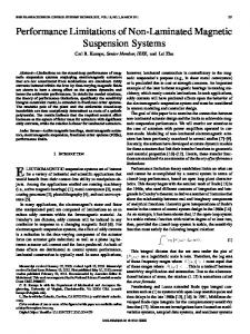
A. Results of the Principle Components’ Sensitivity-Analysis-Based Extraction Procedure Table II contains the percentage error made in the final values of the model elements for both tests for the two transistor examples defined in Table I. Both the maximum and mean error are provided. The accuracy of the method is clear. A novel representation of the performance of the algorithm is shown in Figs. 6 and 7. The -axes represent 100 extractions performed during the tests, while the -axes represent the element values. Each circle shows the starting value for that particular element for one search, while the solid line shows
Fig. 7. Converge diagram and histogram for model elements Ri and Rg for test one. Circles indicate the starting values for each extraction and the solid line the final values.
the final value. Ideally, one should see a perfect horizontal line for the final values, representing no variation in the extracted value. The variation of the solid line from the perfect straight line gives a clear graphical view of the sensitivity of the final values to the starting values. Results are presented for the first test for two dominant and ) and for the two least sensitive model elements ( elements ( and ) for transistor one. The channel resistance and the parasitic gate resistance are of particular interest because of their positions in the model and their electrical equivalence. This makes the determination of their individual values very difficult [8]. A study of the information obtained from various extraction examples revealed the following. 1) Not all parameter-extraction problems can be solved with equal accuracy. This is similar to conclusions reached by Curtise [1]. , could be 2) All the parameters, with the exception of extracted with high accuracy.
VAN NIEKERK AND MEYER: DECOMPOSITION-BASED PARAMETER-EXTRACTION PROCEDURES
TABLE III THE AVERAGE AND MAXIMUM % ERROR IN 100 EXTRACTIONS THE 13-ELEMENT FET MODEL FROM PERFECT AND NOISY DATA WHEN Rg IS FIXED AT ITS CORRECT VALUE
1625
OF
Fig. 8. The distribution of the model elements Cgs and Ri when the second robustness test is done with the parameter Rg fixed at its correct value. The distribution of the element values is now Gaussian.
3) The accuracy with which the parasitic resistances and and the channel resistance could be found varied from example to example. 4) Most of the extracted element values occur in a very narrow range around the correct value. However, from the histograms, it can be observed that the lowest concentration of extracted-parameter values occurs in the middle (near the correct element value) of the distribution, which is somewhat contrary to the behavior of normal statistical processes. The unexpected distribution is also observed in the results of the second robustness test where noise is added to the simulated measurements. Although the added noise has a Gaussian magnitude distribution, the distribution of the parameter values is decidedly non-Gaussian. The following two mechanisms are mainly responsible for this phenomenon. 1) The Distribution of Local Minima Close to the Global Minimum: This is a phenomena that is dependent on the shape of the multidimensional error function, and it cannot be described using statistical methods [10]. As these minima are very close to the global minimum, one can expect the algorithm to converge to these minima more often than to the correct value. 2) The Low Level of Added Noise: These perturbations can be described with statistical distributions, but in order for the histograms of the extracted element values to reflect these distributions, the noise has to be the dominant factor that causes extraction errors. The second test also illustrates that the uncertainty in the determination of the less dominant parameters greatly increases in the presence of imperfections in the data. This , , , and is especially true for the parasitic resistances the channel resistance . is the model element that is the most difficult to determine because of the small influence it has on the value to of the global-error function. This causes the value of
TABLE IV THE AVERAGE AND MAXIMUM % ERROR IN 100 EXTRACTIONS OF 13 ELEMENT FET MODEL FROM PERFECT DATA USING [6], FOR Rg BOTH FREE AND FIXED AT ITS CORRECT VALUE
THE
be obscured by measurement uncertainty and the small errors made in the extraction of the other model elements. Due to this, there is no correlation between the value of the global. error function and the error made in the extraction of is Despite this, Novotny and Kompa [11] found that when fixed at its correct value, and there is a large increase in the overall extraction accuracy. Table III shows the results of the fixed at its correct value, robustness tests performed with while Fig. 8 shows the distributions of the extracted values and for transistor two. It should be for the elements noted that the distributions are now Gaussian, indicating that the influence of the local minima has been greatly reduced. B. Experimental Results for the Algorithm of Kondoh [6] The first robustness test was also performed on the original as algorithm proposed by Kondoh. The test was done with fixed at part of the optimization problem and repeated with its correct value. Table IV contains the results. Figs. 9 and 10
1626
IEEE TRANSACTIONS ON MICROWAVE THEORY AND TECHNIQUES, VOL. 46, NO. 11, NOVEMBER 1998
the extraction accuracy obtained for both methods, but it does not prevent the sensitive elements from getting stuck in local minima for the Kondoh algorithm. Although the extraction accuracy obtained with [6] is still very high for most of the extractions in test one, the procedure is not as robust or accurate as the new adaptive optimization sequence. VII. CONCLUSION
Fig. 9. Convergence diagram and histograms for the first robustness test using the Kondoh algorithm for Cgs and .
Rigorous test results have been presented for the new adaptive decomposition-based optimization procedure proposed in [5]. The results show the accuracy and insensitivity of the parameter extractor to optimization starting values. Robustness tests were performed on the procedure using user-defined data, allowing an absolute level of accuracy to be determined. The tests show that care has to be taken when presenting the extraction results since normal statistical descriptions such as mean and standard deviation may not be appropriate due to the shape of the histograms. The tests also has on the confirm the large influence that the element extraction accuracy that can be obtained and the difficulty of determining this element from only one set of measured parameters. The convergence of the new procedure and the role this plays in the improved robustness of this method have been discussed. The results presented in this paper has been generated with in-house software written in FORTRAN 77 and compiled on a variety of systems. Executing the program on an SGI Power Indigo workstation with a 195-MHz R10000 processor typically took about 16 s for one extraction. REFERENCES
Fig. 10. Convergence diagram and histograms for the first robustness test using the Kondoh algorithm for Ri and Rg .
provides a graphical representation of the extraction results for and , and for the two insensitive the dominant elements and for transistor one. It can clearly be seen elements gets caught in local minima for quite a number of that starting values. Although not being the least sensitive element in the model, is optimized last in the sequence proposed to be by Kondoh. This has the added effect of causing determined incorrectly. The results summarized in Table IV can be misleading. The algorithm described in [6] can provide accurate extractions, but due to the fact that it is more susceptible to local minima, it gets caught far from the correct solution more often. This leads to a higher average error. A comparison of the results in Table IV and Figs. 9 and 10 with those presented in Table II and Figs. 6 and 7 reveals the following: the sensitive elements of the model that are placed low down in the optimization sequence in [6] is more likely to get caught in local minima than in the new algorithm. This will also cause the insensitive elements to be at its correct value improves determined incorrectly. Fixing
[1] W. R. Curtise and R. L. Camisa, “Self-consistent GaAs FET models for amplifier design and device diagnostics,” IEEE Trans. Microwave Theory Tech., vol. MTT-32, pp. 1573–1578, Dec. 1984. [2] G. Dambrine, A. Cappy, F. Heliodore, and E. Playez, “A new method for determining the FET small-signal equivalent circuit,” IEEE Trans. Microwave Theory Tech., vol. 36, pp. 1151–1159, July 1988. [3] F. Lin and G. Kompa, “FET model parameter extraction based on optimization with multiplane data-fitting and bidirectional search—A new concept,” IEEE Trans. Microwave Theory Tech., vol. 42, pp. 1114–1121, July 1994. [4] K. Shirakawa, H. Oikawa, T. Shimura, Y. Kawasaki, Y. Ohashi, T. Saito, and Y. Daido, “An approach to determining an equivalent circuit for HEMT’s,” IEEE Trans. Microwave Theory Tech., vol. 43, pp. 499–503, Mar. 1995. [5] C. van Niekerk and P. Meyer, “A new approach for the extraction of an FET equivalent circuit from measured S -parameters,” Microwave Opt. Technol. Lett., vol. 11, no. 5, pp. 281–284, Apr. 1996. [6] H. Kondoh, “An accurate FET modeling from measured S -parameters,” in IEEE MTT-S Symp. Dig., Baltimore, MD, June 1986, pp. 377–380. [7] J. W. Bandler and Q.-J. Zhang, “An automatic decomposition approach to optimization of large microwave systems,” IEEE Trans. Microwave Theory Tech., vol. MTT-35, pp. 1231–1239, Dec. 1987. [8] A. D. Patterson, V. F. Fusco, J. J. McKeown, and J. A. C. Stewart, “A systematic optimization strategy for microwave device modeling,” IEEE Trans. Microwave Theory Tech., vol. 41, pp. 395–405, Mar. 1993. [9] S. Haykin, Adaptive Filter Theory, 3rd ed. Englewood Cliffs, NJ: Prentice-Hall, 1996. [10] W. H. Press, B. P. Flannery, S. A. Teukolsky, and W. T. Vetterling, Numerical Recipes in C—The Art of Scientific Computing. Cambridge, U.K.: Cambridge Univ. Press, 1988. [11] G. Kompa and M. Novotny, “Highly consistent FET model parameter extraction based on broadband S -parameter measurements,” in IEEE MTT-S Symp. Dig., Albuquerque, NM, 1992, pp. 293–296.
VAN NIEKERK AND MEYER: DECOMPOSITION-BASED PARAMETER-EXTRACTION PROCEDURES
Cornell van Niekerk (S’96) was born in Swellendam, South Africa, in 1971. He received the B.Ing. and M.Eng. degrees from the University of Stellenbosch, Stellenbosch, South Africa, in 1993 and 1996, and is currently working toward the Ph.D. degree, involved with the problem of experimental MESFET model extraction. In 1998, he joined the staff at the Department of Electrical and Electronic Engineering, University of Stellenbosch, where he is currently a Lecturer. His current research interests are the extraction of transistor CAD models, cryogenic circuits, and hybrid high-temperature superconductor circuits.
1627
Petrie Meyer (S’87–M’88) received the M.Eng. and Ph.D. (Eng.) degrees from the University of Stellenbosch, Stellenbosch, South Africa, in 1986 and 1995, respectively. In 1988, he joined the Department of Electrical and Electronic Engineering, University of Stellenbosch, where he is currently a Senior Lecturer. His main interests include hybrid numerical electromagnetic (EM) techniques, with specific attention to the method-of-lines and mode-matching techniques, passive microwave circuits, and design algorithms. Dr. Meyer has served as chair for the IEEE South African Section in 1997, and as technical chair for the 1999 IEEE Region 8 AFRICON Conference.