parameter estimation error at a rate dictated by the closed-loop system's excitation. ... first is the identification of parameters as a part of state observer while the ...
10 Advances in Parameter Estimation and Performance Improvement in Adaptive Control Veronica Adetola and Martin Guay
Department of Chemical Engineering, Queen's University Kingston Canada 1. Introduction In most adaptive control algorithms, parameter estimate errors are not guaranteed to converge to zero. This lack of convergence adversely affects the global performance of the algorithms. The effect is more pronounced in control problems where the desired reference setpoint or trajectory depends on the system's unknown parameters. This paper presents a parameter estimation routine that allows exact reconstruction of the unknown parameters in finite-time provided a given excitation condition is satisfied. The robustness of the routine to an unknown bounded disturbance or modelling error is also shown. To enhance the applicability of the finite-time (FT) identification procedure in practical situations, a novel adaptive compensator that (almost) recover the performance of the FT identifier is developed. The compensator guarantees exponential convergence of the parameter estimation error at a rate dictated by the closed-loop system's excitation. It was shown how the adaptive compensator can be used to improve upon existing adaptive controllers. The modification provided guarantees exponential stability of the parametric equilibrium provided the given PE condition is satisfied. Otherwise, the original system's closed-loop properties are preserved. The results are independent of the control structure employed. The true parameter value is obtained without requiring the measurement or computation of the velocity state vector. Moreover, the technique provides a direct solution to the problem of removing auxiliary perturbation signals when parameter convergence is achieved. The effectiveness of the proposed methods is illustrated with simulation examples. There are two major approaches to online parameter identification of nonlinear systems. The first is the identification of parameters as a part of state observer while the second deals with parameter identification as a part of controller. In the first approach, the observer is designed to provide state derivatives information and the parameters are estimated via estimation methods such as least squares method [19] and dynamic inversion [6]. The second trend of parameter identification is much more widespread, as it allows identification of systems with unstable dynamics. Algorithms in this area include parameter identification methods based on variable structure theory [22, 23] and those based on the notion of passivity [13]. In the conventional adaptive control algorithms, the focus is on the tracking of a given reference trajectory and in most cases parameter estimation errors are not guaranteed to
190
Frontiers in Adaptive Control
converge to zero due to a lack of excitation [10]. Parameter convergence is an important issue as it enhances the overall stability and robustness properties of the closed-loop adaptive systems [14]. Moreover, there are control problems whereby the reference trajectory is not known a priori but depends on the unknown parameters of the system dynamics. For example, in adaptive extremum seeking control problems, the desired target is the operating setpoint that optimizes an uncertain cost function [8, 21]. Assuming the satisfaction of appropriate excitation conditions, asymptotic and exponential parameter convergence results are available for both linear and nonlinear systems. Some lower bounds which depends (nonlinearly) on the adaptation gain and the level of excitation in the system have been provided for some specific control and estimation algorithms [11, 17, 20]. However, it is not always easy to characterize the convergence rate. Since the performance of any adaptive extremum seeking control is dictated by the efficiency of its parameter adaptation procedure. This chapter presents a parameter estimation scheme that allows exact reconstruction of the unknown parameters in finitetime provided a given persistence of excitation (PE) condition is satisfied. The true parameter estimate is recovered at any time instant the excitation condition is satisfied. This condition requires the integral of a filtered regressor matrix to be invertible. The finite-time (FT) identification procedure assumes the state of the system x(⋅) is accessible for measurement but does not require the measurement or computation of the velocity state vector x& (⋅) . The robustness of the estimation routine to bounded unknown disturbances or modeling errors is also examined. It is shown that the parameter estimation error can be rendered arbitrarily small for a sufficiently large filter gain. A common approach to ensuring a PE condition in adaptive control is to introduce a perturbation signal as the reference input or to add it to the target setpoint or trajectory. The downside of this approach is that a constant PE deteriorates the desired tracking or regulation performance. Aside from the recent results on intelligent excitation signal design [3, 4], the standard approach has been to introduce such PE signal and remove it when the parameters are assumed to have converged. The fact that one has perfect knowledge of the convergence time in the proposed framework allows for a direct and immediate removal of the added PE signal. The result on finite-time identification has been published in [2]. The main drawback of the finite-time identification algorithm is the requirement to check the invertibility of a matrix online and compute the inverse matrix when appropriate. To avoid these concerns and enhance the applicability of the FT method in practical situations, the procedure was employed to develop a novel adaptive compensator that (almost) recover the performance of the FT identifier. The compensator guarantees exponential convergence of the parameter estimation error at a rate dictated by the closed-loop system's excitation. It was shown how the adaptive compensator can be used to improve upon existing adaptive controllers. The modification provided guarantees exponential stability of the parametric equilibrium provided the given PE condition is satisfied. Otherwise, the original system's closed-loop properties are preserved.
2. Problem Description and Assumptions The system considered is the following nonlinear parameter affine system (1)
Advances in Parameter Estimation and Performance Improvement in Adaptive Control
191
where is the state and is the control input. The vector is the unknown parameter vector whose entries may represent physically meaningful unknown model parameters or could be associated with any finite set of universal basis functions. It is . assumed that is uniquely identifiable and lie within an initially known compact set The nx-dimensional vector f(x, u) and the -dimensional matrix are bounded and continuous in their arguments. System (1) encompasses the special class of linear systems,
where Ai and Bi for i = 0 . . . are known matrices possibly time varying. Assumption 2.1 The following assumptions are made about system (1). 1. The state of the system x(⋅) is assumed to be accessible for measurement. 2.
There is a known bounded control law and a bounded parameter update law that achieves a primary control objective. The control objective can be to (robustly) stabilize the plant and/or to force the output to track a reference signal. Depending on the structure of the system (1), adaptive control design methods are available in the literature [12, 16]. For any given bounded control and parameter update law, the aim of this chapter is to provide the true estimates of the plant parameters in finite-time while preserving the properties of the controlled closed-loop system.
3. Finite-time Parameter Identification Let
denote the state predictor for (1), the dynamics of the state predictor is designed as (2)
where
is a parameter estimate generated via any update law , kw > 0 is a design matrix, is the prediction error and w is the output of the filter (3)
Denoting the parameter estimation error as
, it follows from (1) and (2) that (4)
The use of the filter matrix w in the above development provides direct information about parameter estimation error without requiring a knowledge of the velocity vector x& . This is achieved by defining the auxiliary variable (5) with , in view of (3, 4), generated from (6) Based on the dynamics (2), (3) and (6), the main result is given by the following theorem.
192
Theorem 3.1 Let
Frontiers in Adaptive Control
and
be generated from the following dynamics: (7a) (7b)
Suppose there exists a time tc and a constant c1 > 0 such that Q(tc) is invertible i.e. (8) then (9) Proof: The result can be easily shown by noting that (10)
. Using the fact that
, it follows from (10) that (11)
and (11) holds for all
since
.
The result in theorem 3.1 is independent of the control u and parameter identifier structure used for the state prediction (eqn 2). Moreover, the result holds if a nominal estimate of the unknown parameter (no parameter adaptation) is employed in the and the last part of the state predictor estimation routine. In this case, is replaced with (2) is dropped ( = 0). Let (12) The finite-time (FT) identifier is given by (13) The piecewise continuous function (13) can be approximated by a smooth approximation using the logistic functions
(14a)
(14b)
193
Advances in Parameter Estimation and Performance Improvement in Adaptive Control
(14c) where larger correspond to a sharper transition at t = tc and An example of such approximation is depicted in Figure 1 where the function
is approximated by (14) with
.
.
Figure 1. Approximation of a piecewise continuous function. The function z(t) is given by the full line. Its approximation is given by the dotted line The invertibility condition (8) is equivalent to the standard persistence of excitation (PE) condition required for parameter convergence in adaptive control. The condition (8) is satisfied if the regressor matrix is PE. To show this, consider the filter dynamic (3), from which it follows that
(15) Since is PE by assumption and the transfer function is stable, minimum phase and strictly proper, we know that w(t) is PE [18]. Hence, there exists tc and a c1 for which (8) is satisfied. The superiority of the above design lies in the fact that the true parameter value can be computed at any time instant tc the regressor matrix becomes positive definite and subsequently stop the parameter adaptation mechanism. The procedure in theorem 42 involves solving matrix valued ordinary differential equations (3, 7) and checking the invertibility of Q(t) online. For computational considerations, the
194
Frontiers in Adaptive Control
invertibility condition (8) can be efficiently tested by checking the determinant of Q(t) online. Theoretically, the matrix is invert-ible at any time det(Q(t)) becomes positive definite. The determinant of Q(t) (which is a polynomial function) can be queried at pre-scheduled times or by propagating it online starting from a zero initial condition. One way of doing this is to include a scalar differential equation for the derivative of det(Q(i)) as follows [7]: (16) where Adjugate(Q), admittedly not a light numerical task, is also a polynomial function of the elements of Q. 3.1 Absence of PE If the PE condition (8) is not satisfied, a given controller and the corresponding parameter estimation scheme preserve the system established closed-loop properties. When a bounded is known, it can be shown that the state controller that is robust with respect to input . An example of such robust controller is an inputprediction error e tends to zero as to-state stable (iss) controller [12]. Theorem 3.2 Suppose the design parameter kw in (2) is replaced with , and . Then the state predictor (2) and the parameter update law (17) with
, a design constant matrix, guarantee that
1. 2. Proof: 1.
. , a constant. Consider a Lyapunov function (18) It follows from equations (4), (5), (6) and (17) that (19) (20) (21) where . This implies uniform boundedness of as well as global asymptotic convergence of to zero. Hence, it follows from (5) that .
2.
This can be shown by noting from (17) that Since (.) and e are bounded signals and finite.
. , the integral term exists and it is
Advances in Parameter Estimation and Performance Improvement in Adaptive Control
195
4. Robustness Property In this section, the robustness of the finite-time identifier to unknown bounded disturbances or modeling errors is demonstrated. Consider a perturbation of
(1): (22) is a disturbance or modeling error term that satisfies . If where the PE condition (8) is satisfied and the disturbance term is known, the true unknown parameter vector is given by (23) with
and the signals
generated from (2), (3) and (24)
respectively. Since is unknown, we provide a bound on the parameter identification error when (6) is used instead of (24). Considering (9) and (23), it follows that (25)
(26) where
is the output of (27)
Since
, it follows that (28)
and hence (29) . where This implies that the identification error can be rendered arbitrarily small by choosing a sufficiently large filter gain . In addition, if the disturbance term and the system satisfies some given properties, then asymptotic convergence can be achieved as stated in the following theorem. , for p = 1 or 2 and , then Theorem 4.1 Suppose asymptotically with time.
196
Frontiers in Adaptive Control
To proof this theorem, we need the following lemma Lemma 4.2 [5]: Consider the system (30) Suppose the equilibrium state xe = 0 of the homogeneous equation is exponentially stable, for , then and 1. if 2. if for p = 1 or 2, then as . Proof of theorem 4.1. It follows from Lemma 4.2.2 that as and therefore is finite. So
(31)
5. Dither Signal Design The problem of tracking a reference signal is usually considered in the study of parameter convergence and in most cases, the reference signal is required to provide sufficient excitation for the closed-loop system. To this end, the reference signal is appended with a bounded excitation signal d(t) as (32) where the auxiliary signal d(t) is chosen as a linear combination of sinusoidal functions with distinct frequencies: (33) where
is the signal amplitude matrix and
is the corresponding sinusoidal function vector. For this approach, it is sufficient to design the perturbation signal such that the regressor matrix is PE. There are very few results on the design of persistently exciting (PE) input signals for nonlinear systems. By converting the closed-loop PE condition to a sufficient richness (SR) condition on the reference signal, attempts have been made to provide verifiable conditions for parameter convergence in some classes of nonlinear systems [3, 1, 14, 15].
Advances in Parameter Estimation and Performance Improvement in Adaptive Control
197
5.1 Dither Signal Removal
Figure 2. Trajectories of parameter estimates. Solid(-) : FT estimates estimates [15]; dashdot(-.): actual value
dashed(--) : standard
Let
denotes the number of distinct elements in the dither amplitude matrix and let be a vector of these distinct coefficients. The amplitude of the excitation signal is specified as (34) or approximated by (35) where equality holds in the limit as
.
198
Frontiers in Adaptive Control
6. Simulation Examples 6.1 Example 1 We consider the following nonlinear system in parametric strict feedback form [15]:
(36)
are unknown parameters. Using an adaptive backstep-ping where design, the control and parameter update law presented in [15] were used for the simulation. The pair stabilize the plant and ensure that the output y tracks a reference signal yr(t) asymptotically. For simulation purposes, parameter values are set to = [—1, —2,1, 2, 3] as in [15] and the reference signal is yr = 1, which is sufficiently rich of order one. The simulation results for zero initial conditions are shown in Figure 2. Based on the convergence analysis procedure in [15], all the parameter estimates cannot converge to their true values for this choice of constant reference. As confirmed in Fig. 2, only 1 and 2 estimates are accurate. However, following the proposed estimation technique and implementing the FT identifier (14), we obtain the exact parameter estimates at t = 17sec. This example demonstrates that, with the proposed estimation routine, it is possible to identify parameters using perturbation or reference signals that would otherwise not provide sufficient excitation for standard adaptation methods. 6.2 Example 2 To corroborate the superiority of the developed procedure, we demonstrate the robustness of the developed procedure by considering system (36) with added exogeneous disturbances as follows:
(37)
where and the tracking signal remains a constant yr = 1. The simulation result, Figure 3, shows convergence of the estimate vector to a small under finite-time identifier with filter gain kw = 1 while no full neighbourhood of parameter convergence is achieved with the standard identifier. The parameter estimation error (t) is depicted in Figure 4 for different values of the filter gain kw . The switching time for the simulation is selected as the time for which the condition number of Q becomes less than 20. It is noted that the time at which switching from standard adaptive estimate to FT estimate occurs increases as the filter gain increases. The convergence performance improves as kw increases, however, no significant improvement is observed as the gain is increased beyond 0.5.
Advances in Parameter Estimation and Performance Improvement in Adaptive Control
199
7. Performance Improvement in Adaptive Control via Finite-time Identification Procedure This section demonstrates how the finite-time identification procedure presented in section 3 can be employed to improve the overall performance (both transient and steady state) of adaptive control systems in a very appealing manner. Fisrt, we develop an adaptive compensator which guarantees exponential convergence of the estimation error provided the integral of a filtered regressor matrix is positive definite. The approach does not involve online checking of matrix in-vertibility and computation of matrix inverse nor switching between parameter estimation methods. The convergence rate of the parameter estimator is directly proportional to the adaptation gain and a measure of the system's excitation. The adaptive compensator is then combined with existing adaptive controllers to guarantee exponential stability of the closed-loop system.
Figure 3. Trajectories of parameter estimates. Solid(-) : FT estimates for the system with additive disturbance , dashed(--): standard estimates [15]; dashdot(-.): actual value
200
Frontiers in Adaptive Control
8. Adaptive Compensation Design Consider the nonlinear system 1 satisfying assumption 2.1 and the state predictor (38) where kw > 0 and
is the nominal initial estimate of . If we define the auxiliary variable (39)
Figure 4. Parameter estimation error for different filter gains kw and select the filter dynamic as (40) then
is generated by (41)
Based on (38) to (41), our novel adaptive compensation result is given in the following theorem. Theorem 8.1 Let Q and C be generated from the following dynamics: (42a) (42b) and let tc be the time such that
, then the adaptation law (43)
201
Advances in Parameter Estimation and Performance Improvement in Adaptive Control
with guarantees that is non-increasing for to and converges to zero exponentially fast, starting from tc. Moreover, the convergence rate is lower . bounded by Proof: Consider a Lyapunov function (44) it follows from (43) that (45) Since
(from (39)), then (46)
and equation (45) becomes (47) (48) This implies non-increase of that shown by noting that
for and the exponential claim follows from the fact is positive definite for all . The convergence rate is
(49) (50) which implies (51) Both the FT identification (9) and the adaptive compensator (43) use the static relationship developed between the unknown parameter and some measurable matrix signals C, i.e, Q = C. However, instead of computing the parameter values at a known finite-time by inverting matrix Q, the adaptive compensator is driven by the estimation error .
9. Incorporating Adaptive Compensator for Performance Improvement It is assumed that the given control law u and stabilizing update law (herein denoted as result in closed-loop error system
)
(52a)
202
Frontiers in Adaptive Control
(52b) is a bounded matrix function where the matrix A is such that and is a vector function of the of the regressor vectors, . This implies that the adaptive controller guarantees tracking error with uniform boundedness of the estimation error and asymptotic convergence of the tracking error Z dynamics. Such adaptive controllers are very common in the literature. Examples include linearized control laws [16] and controllers designed via backstepping [12, 15]. Given the stabilizing adaptation law , we propose the following update law which is a combination of the stabilizing update law (52b) and the adaptive compensator (43) (53) Since C(t) = Q(t) , the resulting error equations becomes (54) Considering the Lyapunov function
and differentating along (54)
we have (55) Hence exponentially for and the initial asymptotic convergence of Z is strengthened to exponential convergence. For feedback linearizable systems
the PE condition translates to a priori verifiable sufficient condition on the reference setpoint. It requires the rows of the regressor vector to be linearly on any finite interval independent along a desired trajectory xr(t) . This condition is less restrictive than the one given in [9] for the same class of system. This is because the linear independence requirement herein is only required over a finite interval and it can be satisfied by a non-periodic reference trajectory while the asymptotic stability result in [9] relies on a T-periodic reference setpoint. Moreover exponential, rather than asymptotic stability of the parametric equilibrium is achieved.
Advances in Parameter Estimation and Performance Improvement in Adaptive Control
203
10. Dither Signal Update Perturbation signal is usually added to the desired reference setpoint or trajectory to guarantee the convergence of system parameters to their true values. To reduce the variability of the closed-loop system, the added PE signal must be systematically removed in a way that sustains parameter convergence. Suppose the dither signal d(t) is selected as a linear combination of sinusoidal functions as be the vector of the selected dither amplitude and let T > 0 be detailed in Section 5. Let the first instant for which d(T) = 0, the amplitude of the excitation signal is updated as follows:
(56) where the gain
is a design parameter,
and
It follows from (56) that the reference setpoint will be subject to PE with constant amplitude if . After which the trajectory of will be dictated by the filtered regressor matrix Q. The amplitude vector will start to decay exponentially when Q(t) becomes positive definite. Note that parameter convergence will be achieved regardless of the value . of the gain selected as the only requirement for convergence is Remark 10.1 The other major approach used in traditional adaptive control is parameter estimation based design. A well designed estimation based adaptive control method achieves modularity of the controller-identifier pair. For nonlinear systems, the controller module must possess strong parametric robustness properties while the identifier module must guarantee certain boundedness properties independent of the control module. Assuming the existence of a bounded controller that is robust with respect to adaptive control design.
, the adaptive compensator (43) serves as a suitable identifier for modular
11. Simulation Example To demonstrate the effectiveness of the adaptive compensator, we consider the example in Section 6 for both the nominal system (36) and the system under additive disturbance (37). The simulation is performed for the same reference setpoint yr = 1, disturbance vector , parameter values = [—1, —2, 1, 2, 3] and zero initial conditions. The adaptive controller presented in [15] is also used for the simulation. We modify the given stabilizing update law by adding the adaptive compensator (43) to it. The modification significantly improve upon the performance of the standard adaptation mechanism as shown in Figures 5 and 6. All the parameters converged to their values and we recover the performance of the finite-time identifier (14). Figures 7 and 8 depict the performance of the output and the input trajectories. While the transient behaviour of the
204
Frontiers in Adaptive Control
output and input trajectories is slightly improved for the nominal adaptive system, a significant improvement is obtained for the system subject to additive disturbances.
Figure 5. Trajectories of parameter estimates. Solid(-) : compensated estimates; dashdot(-.): FT estimates; dashed(--) : standard estimates [15]
Advances in Parameter Estimation and Performance Improvement in Adaptive Control
Figure 6. Trajectories of parameter estimates under additive disturbances. Solid(-): compensated estimates; dashdot(-.): FT estimates; dashed(--) : standard estimates [15]
205
206
Frontiers in Adaptive Control
Figure 7. Trajectories of system's output and input for different adaptation laws. Solid(-): compensated estimates; dashdot(-.): FT estimates; dashed(--) : standard estimates [15]
Figure 8. Trajectories of system's output and input under additive disturbances for different adaptation laws. Solid(-) : compensated estimates; dashdot(-.): FT estimates; dashed(--) : standard estimates [15]
Advances in Parameter Estimation and Performance Improvement in Adaptive Control
207
12. Conclusions The work presented in this chapter transcends beyond characterizing the parameter convergence rate. A method is presented for computing the exact parameter value at a finite-time selected according to the observed excitation in the system. A smooth transition from a standard estimate to the FT estimate is proposed. In the presence of unknown bounded disturbances, the FT identifier converges to a neighbourhood of the true value whose size is dictated by the choice of the filter gain. Moreover, the procedure preserves the system's established closed-loop properties whenever the required PE condition is not satisfied. We also demonstrate how the finite-time identification procedure can be used to improve the overall performance (both transient and steady state) of adaptive control systems in a very appealing manner. The adaptive compensator guarantees exponential convergence of the estimation error provided a given PE condition is satisfied. The convergence rate of the parameter estimator is directly proportional to the adaptation gain and a measure of the system's excitation. The adaptive compensator is then combined with existing adaptive controllers to guarantee exponential stability of the closed-loop system. The application reported in Section 9 is just an example, the adaptive compensator can easily be incorporated into other adaptive control algorithms.
13. References V. Adetola and M. Guay. Parameter convergence in adaptive extremum seeking control. Automatica, 43(1):105-110, 2007. [1] V. Adetola and M. Guay. Finite-time parameter estimation in adaptive control of nonlinear systems. IEEE Transactions on Automatic Control, 53(3):807-811, 2008. [2] V.A. Adetola and M. Guay. Excitation signal design for parameter convergence in adaptive control of linearizable systems. In Proceedings of the 45th IEEE Conference on Decision and Control, San Diego, CA, USA, 2006. [3] Chengyu Cao, Jiang Wang, and N. Hovakimyan. Adaptive control with unknown parameters in reference input. In Proceedings of the 2005 IEEE International Symposium on, Mediterrean Conference on Control and Automation, pages 225—230, June 2005. [4] C.A. Desoer and M. Vidyasagar. Feedback Systems: Input-Output Properties. Academic Press, New York, 1975. [5] F. Floret-Pontet and F. Lamnabhi-Lagarrigue. Parameter identification and state estimation for continuous-time nonlinear systems. In American Control Conference, 2002. Proceedings of the 2002, volume 1, pages 394-399vol. 1, 8-10 May 2002. [6] M. A. Golberg. The derivative of a determinant. The American Mathematical Monthly, 79(10):1124-1126, 1972. [7] M. Guay, D. Dochain, and M. Perrier. Adaptive extremum seeking control of continuous stirred tank bioreactors with unknown growth kinetics. Automatica, 40:881-888, 2004. [8] Jeng Tze Huang. Sufficient conditions for parameter convergence in linearizable systems. IEEE Transactions on Automatic Control, 48:878 - 880, 2003. [9] P.A loannou and Jing Sun. Robust Adaptive Control. Pentice Hall, Upper Saddle River, New Jersey, 1996. [10]
208
Frontiers in Adaptive Control
Gerhard Kreisselmeier. Adaptive observers with exponential rate of convergence. IEEE Transactions on Automatic Control, 22:2—8, 1977. [11] M. Krstic, I. Kanellakopoulos, and P. Kokotovic. Nonlinear and Adaptive Control Design. John Wiley and Sons Inc, Toronto, 1995. [12] I. D. Landau, B. D. O. Anderson, and F. De Bruyne. Recursive identification algorithms for continuous-time nonlinear plants operating in closed loop. Automatica, 37(3):469475, March 2001. [13] Jung-Shan Lin and loannis Kanellakopoulos. Nonlinearities enhance parameter convergence in output-feedback systems. IEEE Transactions on Automatic Control, 43:204-222, 1998. [14] Jung-Shan Lin and loannis Kanellakopoulos. Nonlinearities enhance parameter convergence in strict feedback systems. IEEE Transactions on Automatic Control, 44:89-94, 1999. [15] Ricardo Marino and Patricio Tomei. Nonlinear Control Design. Prentice Hall, 1995. [16] Riccardo Marino and Patrizio Tomei. Adaptive observers with arbitrary exponential rate of convergence for nonlinear systems. IEEE Transactions on Automatic Control, 40:13001304, 1995. [17] K.S Narendra and A.M Annaswamy. Stable and Adaptive Systems. Prentice Hall New Jersey, 1989. [18] Marc; Niethammer, Patrick Menold, and Frank Allgower. Parameter and derivative estimation for nonlinear continuous-time system identification. In 5th IFAC Symposium Nonlinear Control Systems (NOLCOS'Ol), Russia, 2001. [19] S. Sastry and Marc Bodson. ADAPTIVE CONTROL Stability, Convergence, and Robustness. Prentice Hall, New Jersey, 1989. [20] H.H. Wang, M Krstic, and G. Bastin. Optimizing bioreactors by extremum seeking. International Journal of Adaptive Control and Signal Processing, 13:651-669, 1999. [21] Jian-Xin Xu and Hideki Hashimoto. Parameter identification methodologies based on variable structure control. International Journal of Control, 57(5):1207-1220, 1993. [22] Jian-Xin Xu and Hideki Hashimoto. VSS theory-based parameter identification scheme for MIMO systems. Automatica, 32(2):279-284, 1996. [23]