Performance Bounds in Feed-Forward Networks under Blind ... - disco

Performance Bounds in Feed-Forward Networks under Blind Multiplexing Jens B. Schmitt, Frank A. Zdarsky, and Ivan Martinovic disco | Distributed Computer Systems Lab University of Kaiserslautern, Germany Technical Report No. 349/06 April 2006 / Revised in July 2006 Abstract Bounding performance characteristics in communication networks is an important and interesting issue. In this study we assume uncertainty about the way dierent ows in a network are multiplexed, we even drop the common FIFO assumption. Under so-called blind multiplexing we derive new bounds for the tractable, yet non-trivial case of feed-forward networks. This is accomplished for pragmatic, but general trac and server models using network calculus. In particular, we derive an end-to-end service curve for a ow of interest under blind multiplexing, establishing what we call the pay multiplexing only once principle. We specify the algorithms necessary to apply this result in a network of blind multiplexing nodes. Since these algorithms may have prohibitive computational costs, we present strategies to reduce the computational eort in a controlled manner such that the quality of the bounds is aected as little as possible. Finally we present some numerical results from a network calculus tool we developed and compare our bounds against the best known bounds for networks of blind multiplexing nodes.

Keywords : Network calculus, aggregate scheduling, deterministic guarantees.

1

1 Introduction Bounding performance characteristics in communication networks is a fundamental issue and has important applications in network design and control. Network calculus, which is a set of relatively new developments that provide deep insights into ow problems encountered in networks of queues [18], provides a deterministic framework for worst-case analysis of delay and backlog bounds. The basic network calculus results pioneered by [9], [10] in the early 1990s, however, implicitly assume some form of per-ow treatment inside the network in that they only apply to tandems of nodes. Large-scale packet-switched networks as the Internet operate on large aggregates of trac and are far-o from supporting any per-ow state operations, as for example, sophisticated per-ow scheduling. Nevertheless, as [18] pointed out in 2001: The state of the art for aggregate multiplexing is surprisingly poor. Since then considerable eorts have been made to address issues related to bounding performance characteristics in networks of aggregate multiplexing: [7] gives a delay bound for general FIFO networks; [15] extends this work to packetized ows; [27] extends it further to nodes that are allowed to time-stamp packets (similar to what had been proposed previously in [12] as a damper); [26] reproduces the bound found in [7] and uses it for ow population-independent admission control; [13], [14] treat the case of feed-forward FIFO networks; [19] investigates the optimal delay bound under FIFO multiplexing; [25] gives additive delay bounds for tree topologies. All of the above work assumes FIFO nodes. However in practice, as nicely argued in [17], many devices cannot be accurately described by a FIFO model because packets arriving at the output queue from dierent input ports may experience dierent delays when traversing a node. This is due to the fact that many networking devices like routers are implemented using input-output buered crossbars and/or multistage interconnections between input and output ports. Hence, packet reordering on the aggregate level is a frequent event (not so on the ow level) and should not be neglected in modelling. Therefore, in this work we drop the FIFO assumption and make essentially no assumptions on the way aggregates are multiplexed at servers, i.e. we assume blind multiplexing [18]: Definition 1: (Blind Multiplexing) If a node multiplexes several ows and the arbitration discipline between the ows accessing the service of the node is assumed to be unknown we call it a blind multiplexing node. Another issue that arises during the investigation of aggregate scheduling is stability, i.e. whether a nite delay bound exists [4], [2]. For general networks of arbitrary topology it is still very much an open research problem under which circumstances a bound on the delay exists at all [18]. In [7] a sucient condition for stability in general networks is given. Yet, for larger networks this puts a heavy constraint on the utilization of the network since the maximum allowable utilization is inversely proportional to the network diameter. At the other end of the spectrum of topologies, we have tandem networks for which network calculus has become famous to deliver tight bounds for any utilization ≤ 1 (mainly building upon the celebrated concatenation theorem [18]). We concentrate on 2

the middle ground between these two extremes: feed-forward networks. Definition 2: (Feed-Forward Network) A network is feed-forward if it is possible to nd a numbering of its links such that for any ow through the network the numbering of its traversed links is an increasing sequence. It is well-known and easy to show that feed-forward networks are stable for any utilization ≤ 1 [18]. While many networks are obviously not feed-forward, many important instances are. Among these:

• switched networks that typically use spanning trees for routing [20], • wireless sensor networks that can often be modelled as a single-sink or multiple-sink topology that is feed-forward, in fact wireless sensor networks have even been proposed as an application eld of network calculus [22], • MPLS multipoint-to-point label-switched paths which also have been tackled using network calculus in [25]. Furthermore, there are very eective techniques to make a general network feedforward. One of the advanced techniques (in comparison to a simple spanning tree) is the so-called turn-prohibition algorithm [23]. The idea of this algorithm is to prohibit a minimum number of so-called turns (pairs of consecutive edges), but not to delete the edges themselves as a spanning tree algorithm would. Turnprohibition achieves considerably higher throughput than spanning trees and remains fairly close to the maximum achievable throughput of general networks of medium size [23]. So we investigate how to compute performance bounds in feed-forward networks of nodes with blind multiplexing under pretty general assumptions about trac and server models. To the best of our knowledge this has not been done before.

2 Network Calculus Background In this section, the necessary background material for the network calculus applied in this report is presented. Furthermore, some additions as they are needed throughout the report are given.

2.1 Network Calculus Basics Network calculus is a min-plus system theory for deterministic queuing systems which builds on the calculus for network delay in [9], [10]. The important concept of minimum service curve was introduced in [11], [21], [5], [16], [1] and the concept of maximum service curve in [12]. The service curve based approach facilitates the ecient analysis of tandem queues where a linear scaling of performance bounds in the number of traversed queues is achieved as elaborated in [8] and referred to also as pay bursts only once phenomenon in [18]. A detailed 3

treatment of min-plus algebra and of network calculus can be found in [3] and [6], [18], respectively. As network calculus is built around the notion of cumulative functions for input and output ows of data, the set of real-valued, non-negative, and widesense increasing functions passing through the origin plays a major role: © ª F = f : R+ → R+ , ∀t ≥ s : f (t) ≥ f (s), f (0) = 0 In particular, the input function F (t) and the output function F ∗ (t), which cumulatively count the number of bits that are input to respectively output from a system S , are ∈ F . Throughout the report, we assume in- and output functions to be continuous in time and space. This is not a major restriction as there are transformations from discrete to continuous models which do not aect the accuracy of the results signicantly [18]. Definition 3: (Min-plus Convolution and Deconvolution) The min-plus convolution respectively deconvolution of two functions f and g are dened to be ½ inf 0≤s≤t {f (t − s) + g(s)} t ≥ 0 (f ⊗ g) (t) = 0 t 0, the output of the ow is at least equal to β(u). Note that any strict service curve is also a service curve. Using those concepts it is possible to derive basic performance bounds on backlog, delay and output: 5

Theorem 3: (Performance Bounds) Consider a system S that oers a minimum service curve β and a maximum service curve β¯. Assume a ow F traversing the system has an arrival curve α. Then we obtain the following performance bounds: Backlog: ∀t : b(t) ≤ (α ® β) (0) =: v(α, β) Delay: ∀t : d(t) ≤ inf {t ≥ 0 : (α ® β) (−t) ¡ ≤ 0}¢ =: h (α, β) Output (arrival curve α∗ for F ∗ ): α∗ ≤ α ⊗ β¯ ® β ¯ =∞ Note that, if the maximum service cannot be bounded, i.e. ∀t > 0 : β(t) (which is the neutral element for the min-plus convolution), we obtain for the output bound α∗ ≤α ® β . One of the strongest results of network calculus (albeit being a simple consequence of the associativity of ⊗) is the concatenation theorem that enables us to investigate tandems of systems as a single system: Theorem 4: (Concatenation Theorem for Tandem Systems) Consider a ow that traverses a tandem of systems S1 and S2 . Assume that Si oers a minimum service curve βi and a maximum service curve β¯i , i = 1, 2 to the ow. Then the concatenation of the two systems oers a minimum service curve β1 ⊗ β2 and a maximum service β¯1 ⊗ β¯2 to the ow. So far we have only covered the tandem network case, the next result factors in the existence of other interfering ows. In particular, it states the minimum service curve available to a ow at a single node under cross-trac from other ows at that node. Theorem 5: (Blind Multiplexing Nodal Service Curves) Consider a node blindly multiplexing two ows 1 and 2. Assume that the node guarantees a strict minimum service curve β and a maximum service β¯ to the aggregate of the two ows. Assume that ow 2 has α2 as an arrival curve. Then

β1 = [β − α2 ]

+

is a service curve for ow 1 if β1 ∈ F . β¯ remains the maximum service curve + + also for ow 1 alone. Here, the [.] operator is dened as [x] = x ∨ 0, where ∨ denotes the maximum operator. Note that we require the minimum service curve to be strict. In [18] an example is given showing that the theorem otherwise would not hold. It is this theorem that we will generalize to a feed-forward network case in Section 4 in such a way that the costs of multiplexing with interfering ows are only paid once, which forms one of the major contributions of this report. As already mentioned there is very profound work on aggregate scheduling in general networks, the most well known result is probably given by [7], later on reproduced and extended by [27], [15]. As the actual delay bound is derived based on a FIFO assumption we only extract the sucient existence condition for a delay bound which is also valid under blind multiplexing: Theorem 6: (Blind Multiplexing in General Networks) Assume a general network of diameter h with any node n providing a sustained rate Rn and n having bounds on the rates of P all incoming trac Cn . Let us dene the node rf utilization for node n as un = n∈f , with rf denoting the sustained rate of Rn a ow f and n ∈ f means that ow f traverses node n. Then a delay bound 6

exists if

_ n

un
Rn }

n

Cn (Cn − Rn ) (h − 1) + Rn

¶

with σ{cond} (x) equals x if cond is true and 1 otherwise.

2.2 Some Additions In this subsection, we give some basic properties furtherly helpful in the network calculus derivations of Section 4. + Lemma 1: (Distributivity of [.] with respect to ∨) Let f, g be two realvalued functions then it applies that +

+

[f ∨ g] = [f ] ∨ [g]

+ +

+

+

Assume there is a t for which [(f ∨ g) (t)] 6= [f (t)] ∨ [g (t)] . Either f (t) > 0 or g(t) > 0 (otherwise both sides are 0), also both cannot be + > 0 (otherwise both sides are equal as the [.] would have no eect). Without + loss of generality assume f (t) > 0 and g(t) ≤ 0, yet then [(f ∨ g) (t)] = + + + [f (t)] = [f (t)] ∨ [g (t)] which contradicts the assumption and thus proves the statement of the lemma. Note however, the min-plus convolution does not distribute with the minimum operator. Proof:

u t Lemma 2:

it applies that

+

(Lower bound on [.] ) Let f, g be two real-valued functions then +

[f + g] (t) ≥ (f + g) (t) · 1{f (t)≥0,g(t)≥0}

where we use the indicator function 1{cond} , which is 1 if cond is true and 0 otherwise. + Proof: Assume the statement does not hold, that means: ∃t : [f + g] (t) < (f + g) (t) · 1{f (t)≥0,g(t)≥0} . Now f (t) and g(t) cannot both be ≥ 0 since otherwise both sides of the inequation are the same. If, however, one of them is < 0 then the right hand side of the inequation is 0 and thus ≤ to the left hand side. Thus the statement must hold.

u t 3 (Commutativity of inf and ∨) Let fi : Rn → R, i = 1, . . . , n. Let S ⊂ R then ( n ) n _ _ → − − inf f ( x ) = inf fi (→ x) i → − → − Lemma n

x ∈S

Proof:

i=1

i=1

x ∈S

On the one hand ( ≤) ( n ) n _ _ → ∈ S : inf − → →) ∀− x f ( x ) ≤ fi (− x 0 i 0 → − x ∈S

i=1

i=1

7

( ⇒→ inf −

x ∈S

n _

) → fi (− x)

( ≤

i=1

n _

i=1

) →) inf fi (− x 0 − → x0 ∈S

on the other hand ( ≥)

→∈S: ∀− x 0

n _ i=1

( ⇒− inf →

x0 ∈S

n _

n _

→) ≥ fi (− x 0

i=1

) →) fi (− x 0

i=1

≥

inf fi → − x ∈S

n _ i=1

→ (− x)

inf fi → − x ∈S

→ (− x)

which proves the statement of the lemma. Lemma 4: (Alternative Denition of Strict Service Curve) The following two statements are equivalent: (i) a system S oers β as a strict service curve to a ow F , (ii) ∀t ≥ 0 : ∃u ≥ 0 : F (t) ≥ F (t − u) + β(u) and t − u is the start of the last backlogged period for F . Here we assume that for any point in time t where the system is not backlogged, the start of the last backlogged period is dened as t itself (i.e. u = 0). Proof: (i) ⇔ during any backlogged period of duration u ≥ 0 the system oers at least service β(u) to the ow F . ⇔ for any time t for which the last backlogged period started at t−u the output of the ow F ∗ satises: F ∗ (t) − F ∗ (t − u) ≥ β(u) ⇔ for any time t for which the last backlogged period started at t−u the output of the ow F ∗ satises: F ∗ (t) ≥ F (t − u) + β(u) ⇔ (ii)

u t

3 Network Calculus with Piecewise Linear Curves To be able to compute performance bounds in networks of blind multiplexing nodes, we need to apply basic network calculus operations like min-plus convolution and deconvolution on the arrival and service curves we encounter in a given scenario. This cannot be done on general functions with arbitrary characteristics but must, of course, eventually be done with specic instances of arrival and service curves. However, a class of functions which is both tractable as well as general enough to express all common candidates is that of piecewise linear functions. Hence, in this section we present for general piecewise linear arrival and service curves basic network calculus operations upon which further on the network analysis will be built in Section 5.

3.1 A Catalog of Useful Functions In the denition of piecewise linear arrival and service curves the following catalog of functions from F is helpful: 8

Auxiliary functions from F ½ +∞ t > T Burst delay functions: δT (t) = 0 t½≤ T rt + b t > 0 Ane function (token bucket): γr,b (t) = 0 t≤0 ½ R(t − T ) t > T Rate latency function: βR,T (t) = 0 t≤T From these functions general piecewise linear function can be constructed W V using the and as we will encounter in the next subsection. Note that, as mentioned in [18], it applies that ∀f ∈ F : (f ⊗ δT ) (t) = f (t − T ). Hence, a convolution with the burst delay function δT results in a shift along the x-axis according to the value of T . Definition 8:

3.2 Choice of Arrival and Service Curves As already discussed focusing on piecewise linear functions as arrival and service curves is no practical restriction, since it is still general enough to cover virtually any realistic case of trac and server models. In particular many investigations make stronger assumptions: for example treating only the case of token buckets as arrival curve and rate latency functions as service curve is a popular simplication of matters.

3.2.1 Arrival Curve Let us assume a piecewise linear concave arrival curve:

α=

n ^

γri ,bi

i=1

On the one hand it is possible to already use such a function as a trac source description in order to be able to closely approximate a source's worst case behaviour. On the other hand, looking at the network analysis we cannot, as we will see when we factor in the maximum service curve, avoid to model arrival curves inside the network as general piecewise linear concave functions. This is due to the fact that they result from the addition of multiple ows induced by the multiplexing of the latter. To assume concavity is no major restriction because, as discussed in [18], non-concave functions (unless they are not subadditive to be accurate) can be improved by pure knowledge of themselves, thus they cannot be tight.

3.2.2 Minimum Service Curve Let us assume a piecewise linear convex minimum service curve:

β=

m _ j=1

9

βRj ,Tj

A piecewise linear convex minimum service curve results from deriving the service curve for a ow of interest at a node that blindly multiplexes this ow with other ows which, as an aggregate, have a piecewise linear concave arrival curve. Again, it might also be useful to model a node's service curve using several linear segments. To assume convexity is not a major restriction, as it might for instance apply if a node also has other duties. Though, in contrast to the arrival curve which is not sensible for non-concave functions (non-sub-additive to be exact), there are potentially sensible non-convex service curves as for example presented in [24], although this is rather uncommon.

3.2.3 Maximum Service Curve Let us assume a piecewise linear almost concave maximum service curve: Ã l ! ^ β¯ = γr˜k ,˜bk ⊗ δL k=1

By almost concave we mean that the curve is only concave for values of t > L and is 0 for values t ≤ L. If L > 0 this models a node that has a certain minimum latency. The piecewise concavity models again the fact that a node may also have other duties. The concavity in contrast to the convexity for the minimum service curve is due to the fact that a best case instead of a worst case perspective has to be taken. Before discussing the required network calculus operations on these curves, we rst make an observation how the output bound of Theorem 3 can be improved under maximum service curves as they are assumed here.

3.3 Tightening the Output Bound Realising that the maximum service curve induces arrival constraints for the output we can improve the output bound from Theorem 3 by the following lemma. (We prove it slightly more generalconcave instead of just piecewise linear concavethan necessary for our purposes.) Lemma 5: (Improvement of Output Bound) Under the same assumptions as in Theorem 3, let additionally L be such that L = sup{t ≥ 0 : β¯ (t) = 0} (L can be regarded as minimum/xed delay for the system), if β¯ ⊗ δ−L is concave then the output bound for any ow R can be calculated as ¡¡ ¢ ¢ ¡ ¢ α∗ = α ⊗ β¯ ® β ⊗ β¯ ⊗ δ−L Proof:

A bound on the system output at time t can be computed as ¡ © ¢ ª β¯ ® β¯ (t) = sup β¯ (t + s) − β¯ (s) s≥0

¯ to be zero for t ≤ L and to be concave for t > L Since we have assumed β(t) this means that the sup is taken on at s = L such that ¡ ¢ ¡ ¢ ¯ + L) = β¯ ⊗ δ−L (t) β¯ ® β¯ (t) = β(t 10

Hence, as β¯ ⊗ δ−L is a bound on the output of the system it is also an arrival ∗ ¡curve for ¢ any output function R of the ∗system. On the other hand, we have α ⊗ β¯ ® β as curve ¡¡ an arrival ¢ ¢ ¡ for any¢R from Theorem 3. Applying Theorem 2 we obtain α ⊗ β¯ ® β ⊗ β¯ ⊗ δ−L as an output bound.

u t

3.4 Network Calculus Operations We now have everything set to examine the network calculus operations we require as basic building blocks for a network analysis. First of all computing output bounds of the ows in the network is an important operation as it allows to separate ows of interest from interfering ows by using Theorem 5 respectively the results we present in Theorem 7. Lemma 4 gives us the general rule to compute the output bound: ¡¡ ¢ ¢ ¡ ¢ α∗ = α ⊗ β¯ ® β ⊗ β¯ ⊗ δ−L Hence, starting from the innermost operation, the convolution of the arrival curve and the maximum service must be determined rst: ! ÃÃ l ! Ã ! l ^ ^ ¯ γ ˜ ⊗ δL = α ⊗ α⊗β =α⊗ γ ˜ ⊗ δL r˜k ,bk

r˜k ,bk

k=1

k=1

¡ ¡ ¢¢ = α ∧ β¯ ⊗ δ−L ⊗ δL =: σ Here we used rst the associativity of ⊗, then rule 4 from Theorem 1. While σ might look complex, it is easy to compute: rst shift the maximum service curve to the left by its latency then take the minimum with the concave arrival curve and shift the result to the right by the latency of the maximum service curve. Next, the deconvolution of the resulting almost concave function σ with the minimum service curve is calculated as:

σ ® β = (σ ⊗ δ−X ) − β (X) =: ζ o dβ where X = supt≥0 dσ (t) ≥ (t) . X must be at one of the inexion points of dt dt σ and β . Note that ζ is concave since always X ≥ L. And nally ζ is convolved with the right-shifted maximum service curve using rule 4 from Theorem 1: ¡ ¢ ¡ ¢ ζ ⊗ β¯ ⊗ δ−L = ζ ∧ β¯ ⊗ δ−L n

So, in terms of the initial curves we receive as an overall result for the output bound: ¡¡¡¡ ¡ ¢¢ ¢ ¢ ¢ ¡ ¢ α∗ = α ∧ β¯ ⊗ δ−L ⊗ δL ⊗ δX − β (X) ∧ β¯ ⊗ δ−L Equipped with this a single node analysis can be accomplished. However, another basic operation consists of using the concatenation theorem to collapse 11

systems in sequence into one large system by calculating their min-plus convolution. So the convolution of piecewise linear minimum and maximum service curves must be computed. For the minimum service curves we can draw upon rule 5 from Theorem 1 as they are piecewise linear convex functions ∈ F . For maximum service curves the next lemma gives us the computation of the minplus convolution of two almost concave function: Lemma 6: (Min-Plus Convolution of Almost Concave Functions) Consider two almost concave piecewise linear functions β¯1 and β¯2 with latencies L1 and L2 , then their min-plus convolution can be computed as follows ¡ ¢ ¡ ¢ β¯1 ⊗ β¯2 = β¯1 ⊗ δ−L1 ∧ β¯2 ⊗ δ−L2 ⊗ δL1 +L2 Proof:

Again we make use of min-plus algebra ¡¡ ¢ ¢ ¡¡ ¢ ¢ β¯1 ⊗ β¯2 = β¯1 ⊗ δ−L1 ⊗ δL1 ⊗ β¯2 ⊗ δ−L2 ⊗ δL2 ¡¡ ¢ ¡ ¢¢ = β¯1 ⊗ δ−L1 ⊗ β¯2 ⊗ δ−L2 ⊗ (δL1 ⊗ δL2 ) ¡¡ ¢ ¡ ¢¢ = β¯1 ⊗ δ−L1 ∧ β¯2 ⊗ δ−L2 ⊗ δL1 +L2

Here we used associativity and commutativity of ⊗ as well as again rule 4 from Theorem 1.

u t

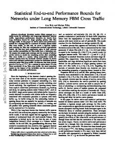
4 The End-to-End Service Curve under Blind Multiplexing Before we come to the actual algorithms for network analysis applying the basic operations that were just presented, we investigate dierent alternatives to derive the end-to-end service curve for a ow of interest through a network of blind multiplexing nodes. One possibility is to derive the end-to-end service curve based on the concatenation theorem and the result for single node blind multiplexing in Theorem 5. This evident method is mentioned in [18]. For example, if a scenario as depicted in Figure 1 is to be analysed for ow 1, a straightforward end-to-end service curve for ow 1 would be determined as follows (using the notation in Figure 1): +

+

β1SF = [β1 − α2 − α3 ] ⊗ [β2 − α2∗ − α3∗ ] ⊗ [β3 − α3∗∗ ]

+

Yet, another way to analyse the system is to concatenate node 1 and 2, subtract ow 2 and thus receive the service curve for ow 1 and 3 together, concatenate this with node 3 and subtract ow 3, essentially making optimal use of the sub-path sharing between the interfering ows:

h i+ + β1P S = [(β1 ⊗ β2 ) − α2 ] ⊗ β3 − α3

12

F3*** ,α 3***

F3 ,α 3 * 3

F ,α

β1

F1 ,α1

F2* ,α 2*

F2 ,α 2

** 3

* 3

F ,α * 1

F ,α

* 1

β2

** 3

F1** ,α1**

β3

F1*** ,α1***

F2** ,α 2**

Figure 1: Nested interfering ows scenario. F3*** ,α 3***

F3 ,α 3 ** 3

F ,α

F1 ,α1 F2 ,α 2

β1 * 2

F ,α

* 2

F1* ,α1*

β2

** 3

F1** ,α1**

β3

F1*** ,α1***

F2** ,α 2**

Figure 2: Overlapping interfering ows scenario. If, for example, βi = β3,0 , i = 1, 2, 3 and α2 = α3 = γ1,1 we obtain: β1SF = β1,12 21 and β1P S = β1,2 . Hence, exploiting the sub-path sharing between the interfering ows, we obtain an end-to-end service curve with considerably lower latency. Put in other words, we have to pay for the blind multiplexing of the ows only once, which is why we also call this phenomenon the pay multiplexing only once (PMOO) principle, in analogy to the well-known pay bursts only once principle [18]. Basically the same observation was made in [13], [14] for FIFO multiplexing under the special case of token bucket arrival curves and rate-latency service curves. We derive the end-to-end service curve for blind multiplexing exploiting the PMOO principle under general piecewise linear concave arrival curves and general piecewise linear convex service curves. The diculty in obtaining the end-to-end service under blind multiplexing for a ow of interest lies in situations as depicted in Figure 2. Here, in contrast to the scenario of nested interfering ows as in Figure 1, we have a scenario of overlapping interfering ows, i.e. ows 2 and 3 which interfere with ow 1, our ow of interest, that share some servers with each other but each also traverses servers the other does not traverse. For such a scenario the endto-end service curve cannot be derived as easily as demonstrated before but requires to look deeper into the input and output relationships of the ows. The following theorem states how to calculate the end-to-end service curve under blind multiplexing exploiting the PMOO principle for the canonical example of overlapping interfering ows in Figure 1. Theorem 7 (End-to-End Minimum Service Curve under Blind Multiplexing  Pay Multiplexing Only Once Principle) Consider a scenario as shown in Figure 2: a ow of interest F1 interfered by two overlapping other ows F2 and F3 . F2 and F3 have arrival curves α2 and α3 . The three servers each oer a strict minimum service curve βi , i = 1, 2, 3. The

13

output ows of each of the servers are denoted as in Figure 2. If α2 = and α3 =

m V j=1

φ=

n V i=1

γri ,bi

γrˆj ,ˆbj are piecewise linear concave arrival curves then

n _ m h ´i+ _ ¡ ¢ ³ (β1 − γ˜ri ,bi ) ⊗ β2 − γri ,0 − γrˆj ,0 ⊗ β3 − γ˜rˆj ,ˆbj i=1 j=1

constitutes a strict end-to-end service curve for the ow½of interest, in particular γr,b (t) t 6= 0 F1∗∗∗ ≥ F1 ⊗ φ. Here we use a new notation: γ˜r,b (t) = . b t=0 Proof: Since β3 is a strict service curve we know from Lemma 4 that ∀t ≥ 0 : ∃u ≥ 0 :

(F1∗∗∗ + F3∗∗∗ ) (t) ≥ (F1∗∗ + F3∗∗ ) (t − u) + β3 (u) and t − u is the start of the last backlogged period at node 3.

=⇒ F1∗∗∗ (t) − F1∗∗ (t − u) ≥ β3 (u) − (F3∗∗∗ (t) − F3∗∗ (t − u))

(1)

Along the same lines we can show for node 2 that ∀(t − u) ≥ 0 : ∃s ≥ 0 : =⇒ F1∗∗ (t − u) − F1∗ (t − u − s) ≥ β2 (s)

− (F2∗∗ (t − u) − F2∗ (t − u − s)) − (F3∗∗ (t − u) − F3∗ (t − u − s))

(2)

and t − u − s is the start of the last backlogged period at node 2 and the composed service at node 3 and 2. And for node 1 that ∀(t − u − s) ≥ 0 : ∃r ≥ 0 : =⇒ F1∗ (t − u − s) − F1∗ (t − u − s − r) ≥ β1 (r)

− (F2∗∗ (t − u − s) − F2∗ (t − u − s − r))

(3)

and t − u − s − r is the start of the last backlogged period at node 1 and and the composed service at node 1,2, and 3. If we add up (1), (2), and (3) we obtain ∀t ≥ 0 : ∃u, s, r ≥ 0 :

F1∗∗∗ (t) − F1 (t − u − s − r) ≥ β1 (r) + β2 (s) + β3 (u) − (F2∗∗ (t − u) − F2 (t − u − s − r)) − (F3∗∗∗ (t) − F3 (t − u − s)) and t − u − s − r is the start of the last backlogged period of the composed service at node 1, 2, and 3. Now using the causality of the systems under observation and the arrival curves for F2 and F3 we arrive at

F1∗∗∗ (t) − F1 (t − u − s − r) ≥ β1 (r) + β2 (s) + β3 (u) −α2 (s + r) − α3 (s + u) 14

≥

inf {β1 (r0 ) + β2 (s0 ) + β3 (u0 ) 0 r ,s ,u ≥ 0 r0 + s0 + u0 = s + u + r 0

0

−α2 (s0 + r0 ) − α3 (s0 + u0 )} =

inf {β1 (r0 ) + β2 (s0 ) + β3 (u0 ) 0 r ,s ,u ≥ 0 r0 + s0 + u0 = s + u + r  n m  ^ ^ − γri ,bi (s0 + r0 ) − γrˆj ,ˆbj (s0 + u0 )  0

0

i=1

=

=

j=1

 n _ m _

inf (β1 (r0 ) + β2 (s0 ) + β3 (u0 )) 0  r ,s ,u ≥ 0 i=1 j=1 r 0 + s0 + u 0 = s + u + r o −γri ,bi (s0 + r0 ) − γrˆj ,ˆbj (s0 + u0 ) 0

n _ m _ i=1 j=1

0

{β1 (r0 ) + β2 (s0 ) + β3 (u0 ) inf r 0 , s 0 , u0 ≥ 0 r0 + s0 + u0 = s + u + r o −γri ,bi (s0 + r0 ) − γrˆj ,ˆbj (s0 + u0 )

(4)

The last equation is due to Lemma 3. Now we need to bring in the special shape of the arrival curves being additively composable. In particular we have ½ γri ,0 (s0 ) + γ˜ri ,bi (r0 ) s0 + r0 > 0 γri ,bi (s0 + r0 ) = 0 s0 + r 0 = 0 ½ γrˆj ,0 (s0 ) + γ˜rˆj ,ˆbj (u0 ) s0 + u0 > 0 γrˆj ,ˆbj (s0 + u0 ) = 0 s0 + u0 = 0 Note that we have dierent equivalent choices for the additive separation of the token buckets. To return to (4) we need to distinguish four cases: Case 1: s0 + r0 > 0 and s0 + u0 > 0 ⇒ s + r > 0 and s + u > 0 ⇒ either s > 0 or r, u > 0. This corresponds to having a non-zero backlog at least at two of the three nodes or at node 2, thus

F1∗∗∗ (t) − F1 (t − u − s − r) ≥

n _ m _

inf {β1 (r0 ) + β2 (s0 ) + β3 (u0 ) 0 r ,s ,u ≥ 0 i=1 j=1 r0 + s0 + u0 = s + u + r o −γri ,0 (s0 ) − γ˜ri ,bi (r0 ) − γrˆj ,0 (s0 ) + γ˜rˆj ,ˆbj (u0 ) 0

0

15

³ ´´´ ⊗ β3 − γ˜rˆj ,ˆbj (u + s + r)   n _ m _ = φi,j  (u + s + r) i=1 j=1

´ ¡ ¢ ³ with φi,j = (β1 − γ˜ri ,bi ) ⊗ β2 − γri ,0 − γrˆj ,0 ⊗ β3 − γ˜rˆj ,ˆbj for i = 1, . . . , n and j = 1, . . . , m. Case 2: s0 +r0 = 0 and s0 +u0 = 0 ⇒ s+r = 0 and s+u = 0⇒ s = r = u = 0. This corresponds to having a non-zero backlog for the composed service at time t = t − u − s − r, thus   n _ m _ F1∗∗∗ (t) − F1 (t − u − s − r) = 0 ≥  φi,j  (0) i=1 j=1 n _ m _

=

³ ´ − bi + ˆbj

i=1 j=1

Case 3: s + r > 0 and s + u = 0 ⇒ s + r > 0 and s + u = 0 ⇒ r > 0 and s = u = 0. This corresponds to having a non-zero backlog only at node 1, thus 0

0

0

0

F1∗∗∗ (t) − F1 (t − u − s − r) ≥

n _

{β1 (r) + γ˜ri ,bi (r)}

i=1

=

n _

 {β1 (r) − ri r − bi } ≥ 

i=1

n _ m _

 φi,j  (r)

i=1 j=1

=

n _ m n o _ β1 (r) − ri r − bi − ˆbj i=1 j=1

Case 4 : s0 + r0 = 0 and s0 + u0 > 0 ⇒ s + r = 0 and s + u > 0⇒ u > 0 and s = r = 0. This corresponds to having a backlog only at node 3, thus (analogous to Case 3 ) F1∗∗∗ (t) − F1 (t − u − s − r) ≥

m n o _ β3 (u) + γ˜rˆj ,ˆbj (u) j=1

 ≥

n _ m _ i=1 j=1

 φi,j  (u) =

n _ m n o _ β3 (u) − rˆj u − ˆbj − bi i=1 j=1

Taking all four cases together we arrive at ∀t ≥ 0 : ∃u, s, r ≥ 0 :   n _ m _  φi,j  (u + s + r) ≤ F1∗∗∗ (t) − F1 (t − u − s − r) i=1 j=1

16

= F1∗∗∗ (t) − F1∗∗∗ (t − u − s − r) The last equality is due to the fact that t − u − s − r is the start of the last backlogged period for the service of the composed system. Since F1∗∗∗ ∈ F we obtain ∀t ≥ 0 : ∃u, s, r ≥ 0 :   + n _ m _ F1∗∗∗ (t) − F1 (t − u − s − r) ≥  φi,j  (u + s + r) i=1 j=1

=

n _ m _

+

[φi,j (u + s + r)] = φ(u + s + r)

i=1 j=1

and t − u − s − r is the start of the last backlogged period of the composed service system. Note that we used Lemma 1 for the last equality. According to Lemma 4 this establishes φ as a strict end-to-end service curve for ow 1.

u t As we are dealing with piecewise linear convex service curves we provide a corresponding application of Theorem 7 in the following corollary: Corollary 1: (PMOO End-to-End Minimum Service Curve under Piecewise Linear Convex Nodal Service Curves) Under the assumptions of Theorem 7, suppose the three servers oer (strict) piecewise linear convex minimum n n ni W Wj Wk service curves β1 = βRi ,Ti , β2 = βRˆ j ,Tˆj , and β3 = βR˜ k ,T˜k . With

α2 =

nl V l=1

i=1

γrl ,bl and α3 = φ=

nV m

j=1

k=1

γrˆm ,ˆbm ,

m=1 ni nj

nk _ nl n m __ _ _

βRi,j,k,l,m ,Ti,j,k,l,m

i=1 j=1 k=1 l=1 m=1

with

³ ´ ³ ´ ˆ j − rl − rˆm ∧ R ˜ k − rˆm Ri,j,k,l,m = (Ri − rl ) ∧ R and

Ti,j,k,l,m = Ti + Tˆj + T˜k ³ ´ ³ ´ bl + ˆbm + rl Ti + Tˆj + rˆm Tˆj + T˜k ³ ´ ³ ´ + ˆ j − rl − rˆm ∧ R ˜ k − rˆm (Ri − rl ) ∧ R

constitutes a strict (piecewise linear convex) end-to-end service curve for the ow of interest, in particular F1∗∗∗ ≥ F1 ⊗ φ. Proof: Substituting the actual service curves into the result from Theorem 7 gives "Ã n ! nl n m _ _ _i φ= βRi ,Ti − γ˜ri ,bi ⊗ l=1 m=1

i=1

17

 



nj _

βRˆ j ,Tˆj − γri ,0 − γrˆj ,0  ⊗

j=1

βR˜ k ,T˜k − γ˜rˆj ,ˆbj

!+ 

k=1 nj nk nl nm ni _ _ _ _ _

= ³

Ãn k _

[(βRi ,Ti − γ˜ri ,bi ) ⊗

i=1 j=1 k=1 l=1 m=1

´i+ ´ ³ βRˆ j ,Tˆj − γri ,0 − γrˆj ,0 ⊗ βR˜ k ,T˜k − γ˜rˆj ,ˆbj =

nj nk nl nm ni _ _ _ _ _

βRi,j,k,l,m ,Ti,j,k,l,m

i=1 j=1 k=1 l=1 m=1

Here the rst equation is due to Lemma 3 and the second equation is an application of Rule 5 from Theorem 1 (note that in Theorem 1 we required the functions to be ∈ F , yet the construction rule also holds for the type of functions we have here).

u t The generalization to an arbitrary number of nodes is notationally complex but follows along the same line of argument as the three nodes with overlapping interference scenario, therefore it is left out here. It had of course to be taken into account for the implementation of the Network Calculator tool that will be described in Section 5. The derivation of the end-to-end maximum service curve is simple and given in the next lemma: Lemma 7: (E2E Maximum Service Curve under Blind Multiplexing) Consider a ow R that traverses a sequence of systems Si , i = 1, . . . , n where it is blindly multiplexed with an arbitrary number of ows. Assume each of the systems oers a nodal maximum service β¯i , ß = 1, . . . , n then ow R is oered

β¯ =

n O

β¯i

i=1

as a maximum service on its path. It is obvious that in the best case R is not interfered at any of the systems Si and thus receives the nodal maximum service curve β¯i at each of its traversed systems such that the overall maximum service curve β follows directly from the basic concatenation result for maximum service curves in Theorem 4.

u t

5 Network Analysis Algorithms In this section, we now present the algorithms to analyse networks of blind multiplexing nodes. We focus on the delay bound computation. The backlog bound computation is analogous and just requires to compute the vertical deviation v where for the delay the horizontal deviation h is calculated. 18

Algorithm 1 Straightforward Network Analysis ComputeDelayBound (ow of interest f )

forall nodes i ∈ path(f ) starting at sink forall pred(i) αpred += ComputeOutputBound(pred(i), {ows to node i from pred(i)}\{f}) + βief f = [βi − αpred ] Nn ef f SF β = ¡i=1 βi ¢ return h αf , β SF

ComputeOutputBound(from node i, ows F)

forall pred(i) αpred + =ComputeOutputBound(pred(i), {ows to node i from pred(i)}∩F) αexcl += ComputeOutputBound(pred(i), {ows to node i from pred(i)}\F) + βief f =³[βi − αexcl ] ´ ¡ ¡ ¢ ¢ return αpred ⊗ β¯i ® β ef f ⊗ β¯i ⊗ δL i

i

5.1 Straightforward Network Analysis This analysis is based on Theorem 5 and the way it is done is described on a high level in Algorithm 1. It consists mainly of two procedures: One to compute the delay bound for the ow of interest using the nodal service curve under blind multiplexing from Theorem 5 and convolving all nodal service curves to nd the end-to-end service curve for the ow of interest which is then used to compute a delay bound for the ow. To be able to compute the nodal service curve, another procedure is required which computes the output bound for all interfering ows at a certain node. This is a recursive procedure which needs to take into account the eect of a general feed-forward network that even ows which never share a server with the ow of interest may aect the ow of interest transitively, by interfering with a ow which in turn interferes with the ow of interest.

5.2 PMOO Network Analysis This analysis is based on Theorem 7 and the way it is done is described in Algorithm 2. It is more complicated than the straightforward analysis and consists of three procedures. The simplest is the one computes the delay bound and uses another procedure to compute the end-to-end service curve for the ow of interest according to Theorem 7. From the result it then calculates the delay bound for the ow of interest. The main complexity lies in the procedure to compute the PMOO service curve. Initially, the path of the ow of interest needs to be prepared to enable an ecient application of the PMOO result. At rst, ows that join the ow of interest several times are eliminated by introducing

19

fresh ows for each later rejoin (with the arrival constraints of the original ow at that node in the network, of course). Next, parallel interfering ows, i.e. ows that have the same ingress and egress nodes, are merged together into a ow set which is treated as one ow for the computation of the service curve. The merging helps to keep the procedure as ecient as possible, since fewer ows have to be taken into account. However, care must be taken when computing the arrival constraints for each of the ow sets, since the ows contained in a set are generally not in parallel throughout the whole network. This is done by a separate procedure which we will discuss in a moment. After the arrival constraints of each of the ow sets have been computed, Theorem 7 is applied to compute the desired end-to-end PMOO service curve. This statement sounds harmless, however the computation of the maximum over all token buckets of the piecewise linear arrival curves of interfering ows and rate-latency functions of the piecewise linear service curve of the nodes on the path of the ow of interest can be a computationally intensive task. We come back to this issue in the next subsection. The last procedure serves to compute the output bound of a ow set behind a given node. Here, the PMOO result is reused as much as possible by rst nding the sub-path shared by all ows in the ow set, respectively the node where the ow set splits. From that split point the procedure recurs on itself for each of the smaller ow sets after the split point. With the sum of those output bounds after the split point, the procedure now calls in indirect recursion the procedure for the computation of the PMOO service curve for the shared path of the ow set. Furthermore, the maximum service curve according to Lemma 6 is calculated. Together, minimum and maximum service curve are applied to calculate the output bound according to Lemma 4.

5.3 Computational Eort Reduction As briey pointed out in the preceding section, the computational eort for the PMOO analysis can be prohibitive as it grows exponentially with the number of interfering ows. This is due to the maximum computation from Theorem 7 that needs to be done for each combination of token buckets of the piecewise linear concave interfering ows and rate latency functions of the servers' piecewise linear convex service curves. Let us assume for this discussion that the nodes use simple rate latency functions such that those do not contribute to the combinatorial explosion. While this assumption will often hold in practice, it is possible, if not even very likely, for the arrival curves of the interfering ows to be composed of several token buckets due to the way the maximum service curve aects the burstiness of ows. Then the number of combinations for the Qf computation of the PMOO service curve equals j=1 nj , where f is the number of interfering ows and nj is the number of token buckets of which interfering ow j is composed. For instance, if all of the arrival curves of interfering ows consist of two token buckets when joining the ow of interest (not when they enter the network), then the number of combination is 2f . The basic PMOO analysis algorithm already reduces the number of combinations by merging parallel ows. This does not aect the computation of the bound. However, we can 20

Algorithm 2 PMOO Network Analysis ComputeDelayBound (ow of interest f )

let p be the path of the ow of interest f β P M OO =¡ ComputePMOOServiceCurve( p, {f }) ¢ return h αf , β P M OO

ComputePMOOServiceCurve(path p, ows F )

eliminate rejoining interfering ows merge parallel interfering ows into owsets Fi forall interfering owsets Fi forall pred(nFi ) of the ingress node nFi of Fi αFi += ComputeOutputBound(pred(nFi ), Fi ) calculate β P M OO using αFi according to Corollary 1 return β P M OO

ComputeOutputBound(from node i, ows F )

nd shared path p of ows in F starting at node i call s the last node on path p (→split point) forall pred(s) αs += ComputeOutputBound(pred(s), {ows to node s from pred(s)}∩F) βpP M OO = ComputePMOOServiceCurve(p, F) calculate β¯pP M OO according to Lemma 6 ¡¡ ¢ ¢ ¡ ¢ return αsplit ⊗ β¯pP M OO ® βpP M OO ⊗ β¯pP M OO ⊗ δLp

go further in reducing the computational eort if we accept some degradation of the PMOO analysis. There are two interesting techniques for directly reducing the computational eort of the maximum operation from Theorem 7 by decreasing the number of combinations to be computed (both can be invoked in procedure ComputeOutputBound in Algorithm 2 just before β P M OO is calculated): Flow Prolongation. The idea of this technique is that ows can be prolonged (of course, only for the analysis) such that they can be merged with other ows. Thus the number of combinations is reduced, for instance, from 2f to 2f −1 for each ow that is prolonged. A ow prolongation incurs some cost as the ow consumes more resources at the servers it now traverses in addition depending on the latency of the servers and the rate of the ow. Often, this cost is small (and zero for a constant rate server). We therefore included that computational reduction technique into our PMOO analysis by accepting all ow prolongations that are below a certain charge starting with the shortest possible. Arrival Curve Approximation. The idea of this technique is to reduce the complexity of the trac descriptions of the interfering ows, i.e. to decrease the nj , without compromising the arrival constraints of the interfering ows. Taken to the extreme we could represent each interfering ow with a 21

single token bucket, the one with the highest bucket depth and the lowest rate which would result in only a single combination that has to be computed. This would certainly be too much computational eort reduction at a potentially high degradation of the bounds. Therefore, we try to eliminate those linear segments from the arrival curves of interfering ows that have the least impact on their shape. To achieve, this we sort all segments in descending order of their y -range and only take a specied number of segments for the further calculation. Note that we do this globally over all segments of arrival curves of interfering ows and not per arrival curve to ensure that over-complex modelling is reduced at the right place. The target number of segments we keep is set to a selectable average number of segments per arrival curve times the number of interfering ows. This allows to reduce the computational eort in a controlled manner while degrading the bounds as little as possible. Apart from these two techniques there is another option: restricting the recursion depth of the output bound computation. That means at a dened recursion depth we stop to use the PMOO-specic procedure to compute the output bound and use the straghtforward analysis specic computation of the output bound instead. The latter avoids the combinatorial explosion from that recursion level on. For example, if the maximum recursion depth is set to 1, then we eectively do not use the PMOO result to compute the output bound but just use it to compute the service curve for the ow of interest.

6 Numerical Experiments To validate and evaluate the proposed methods for computing performance bound in blind multiplexing networks we have implemented a toolbox called DISCO Network Calculator. This toolbox is more generally usable than just for the analysis of networks of blind multiplexing nodes. For instance, we have also implemented FIFO service curves for general piecewise concave arrival curves and piecewise linear convex service curves. The DISCO Network Calculator, which is written in JavaT M , is publicly available1 and may hopefully be of use for other researchers interested in network calculus.

6.1 Experimental Design In order to create a representative network we used the BRITE topology generator with the following recommended parameter settings: 2-level-top-down topology type with 10 ASes with 10 routers each, Waxman's model with α = 0.15, β = 0.2, and random node placement with incremental growth type. The diameter of the generated topology is 11 hops. Hosts are created randomly at access routers: 30% random routers in each AS get a uniform random number of hosts between 1 and 5. This topology is then transformed into a feed-forward network using the turn-prohibition algorithm. The turn-prohibition algorithm resulted in a change 1 http://disco.informatik.uni-kl.de/content/Downloads

22

of 13% of the shortest path routes with an average change of 1.9 hops and a standard deviation of 1.2. So, altogether the routes were changed only by 0.25 hops on average. This can be considered a success for the turn-prohibition algorithm, because it was able to transform this general network with a diameter of 11 into a feed-forward network. Thus it is now suitable to be analysed by the methods presented in Section ?? for all possible network utilizations ≤ 1, whereas if it had been analysed as a general network using, e.g., the bound from [7] it could have been analysed only for utilizations below 10% (according to Theorem 2.1), so we are in a much better position now without paying a high cost in excessive route prolongation. Now, for each source a ow is generated towards a randomly assigned sink. Each ow's arrival curve is drawn from a set Sα of candidate arrival curves. Specically, for this investigation we restricted the set members to token buckets. The minimum service curves were restricted to be rate-latency functions. These provide 1 of 3 rates: C , 2C , or 3C , where C is chosen such that the most loaded link can carry its load (plus a margin of 10%) and for the other links the rate is chosen closest to their carried load. The latency is chosen to be 10ms networkwide. If a maximum service curve is used its latency is set to zero and its rate equal to the rate of the corresponding nodal minimum service curve.

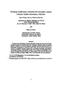
6.2 PMOO Analysis vs. Straightforward Analysis One of the goals of the more comprehensive this study in was to nd out how the straightforward analysis and the PMOO analysis compare to each other. We perform this comparison © ª for two dierent trac scenarios, one with low burstiness (Sα = γr,0.05[s]r , with ©r = 10 Mbit/s) and the other one with ª signicantly higher burstiness (Sα = γr,0.05[s]r , γr,0.25[s]r , γr,0.5[s]r , with r = 10 Mbit/s). Furthermore, we want to isolate the eects by (1) the service curve computation using the PMOO principle, (2) the output bound computation using the PMOO principle, and (3) the maximum service curve in its improved version according to Lemma 3.3. We use all available sinks for ow generation and compute 10 replications with dierent seeds. The results can be found in Figure 3. First we take a look at the eect of the PMOO service curve alone: It is considerably better than its straightforward counterpart for both low and high burstiness of the trac. As expected, the burstier trac incurs higher absolute delays, but the percentage of improvement is roughly the same for both types of ows: ≈ 66 ± 6.5% at a 95% level of condence. When the PMOO output bound is used this gives a further signicant improvement of ≈ 13% for the PMOO analysis (for both trac types). When the maximum service curve is used this reduces the bounds by another ≈ 16%. The maximum service curve also improves the straighforward analysis by ≈ 35% (low) and ≈ 45% (high) and thus keeps its promise to be valuable for a good delay bound analysis although it leads to more complex models.

23

40 SFA PMOOA

35

delay bound [s]

30 25 20 15 10 5 0 low

high

Standard OB, no Max SC

low

high

PMOO-OB, no Max SC

low

high

PMOO-OB, Max SC

Figure 3: PMOO analysis vs. straighforward analysis in turn-prohibited networks.

7 Conclusion In this report, we have presented a comprehensive set of methods to address the issue of computing performance bounds in feed-forward networks under blind multiplexing assumptions. Starting from the derivation of the basic operations for piecewise linear arrival and service curves required for the network analysis, we derived an interesting result on a novel way to compute the end-to-end service curve for a ow of interest under blind multiplexing, again for the pretty general case of piecewise linear arrival and service curves. Equipped with these results we presented algorithms for the network analysis for a straightforward technique based on existing results and a technique based on our new results. We demonstrated that in realistic environments the new bounds can be signicantly better, reducing the existing bounds by at least 50% in our scenarios. A drawback of these bounds is their potentially high computational eort if the model sophistication is high, i.e. either sources have already complicated trac descriptions or maximum service curves generate complex trac ows inside the network. While often in theory such complexities are avoided due to their inelegance this may lead to much looser bounds than necessary. In fact, we are quite happy with our approach of allowing that complexity during the modelling phase and only during the computation of the bounds the complexity is reduced in a way to minimally impact the quality of the bounds.

References [1] R. Agrawal, R. L. Cruz, C. Okino, and R. Rajan. Performance bounds for ow control protocols. IEEE/ACM Transactions on Networking, 7(3):310 323, June 1999.

24

[2] M. Andrews. Instability of fo in session-oriented networks. In Proc. SODA, pages 440447, March 2000. [3] F. Baccelli, G. Cohen, G. J. Olsder, and J.-P. Quadrat. Synchronization and Linearity: An Algebra for Discrete Event Systems. Probability and Mathematical Statistics. John Wiley & Sons Ltd., West Sussex, Great Britain, 1992. [4] C.-S. Chang. Stability, queue length and delay of deterministic and stochastic queueing networks. IEEE Transactions on Automatic Control, 39(5):913931, May 1994. [5] C.-S. Chang. On deterministic trac regulation and service guarantees: A systematic approach by ltering. IEEE Transactions on Information Theory, 44(3):10971110, May 1998. [6] C.-S. Chang. Performance Guarantees in Communication Networks. Telecommunication Networks and Computer Systems. Springer-Verlag, London, Great Britain, 2000. [7] A. Charny and J.-Y. Le Boudec. Delay bounds in a network with aggregate scheduling. In Proc. QofIS, pages 113, September 2000. [8] F. Ciucu, A. Burchard, and J. Liebeherr. A network service curve approach for the stochastic analysis of networks. In Proc. ACM SIGMETRICS, pages 279290, June 2005. [9] R. L. Cruz. A calculus for network delay, Part I: Network elements in isolation. IEEE Transactions on Information Theory, 37(1):114131, January 1991. [10] R. L. Cruz. A calculus for network delay, Part II: Network analysis. IEEE Transactions on Information Theory, 37(1):132141, January 1991. [11] R. L. Cruz. Quality of service guarantees in virtual circuit switched networks. IEEE Journal on Selected Areas in Communications, 13(6):1048 1056, August 1995. [12] R. L. Cruz. SCED+: Ecient management of quality of service guarantees. In Proc. IEEE INFOCOM, volume 2, pages 625634, March 1998. [13] M. Fidler. Extending the network calculus pay bursts only once principle to aggregate scheduling. In Proc. QoS-IP, pages 1934, February 2003. [14] M. Fidler and V. Sander. A parameter based admission control for dierentiated services networks. Computer Networks, 44(4):463479, 2004. [15] Y. Jiang. Delay bounds for a network of guaranteed rate servers with fo aggregation. Computer Networks, 40(6):683694, 2002.

25

[16] J.-Y. Le Boudec. Application of network calculus to guaranteed service networks. IEEE Transactions on Information Theory, 44(3):10871096, May 1998. [17] J.-Y. Le Boudec and A. Charny. Packet scale rate guarantee for non-fo nodes. In Proc. IEEE INFOCOM, pages 2326, June 2002. [18] J.-Y. Le Boudec and P. Thiran. Network Calculus A Theory of Deterministic Queuing Systems for the Internet. Number 2050 in Lecture Notes in Computer Science. Springer-Verlag, Berlin, Germany, 2001. [19] L. Lenzini, E. Mingozzi, and G. Stea. Delay bounds for fo aggregates: A case study. In Proc. QofIS, pages 3140, February 2003. [20] Radia Perlman. Interconnections (2nd ed.): bridges, routers, switches, and internetworking protocols. Addison-Wesley Longman Publishing Co., Inc., Boston, MA, USA, 2000. [21] H. Sariowan, R. L. Cruz, and G. C. Polyzos. Scheduling for quality of service guarantees via service curves. In Proc. IEEE ICCCN, pages 512 520, September 1995. [22] J. Schmitt and U. Roedig. Sensor network calculus - a framework for worst case analysis. In Proc. DCOSS, pages 141154, June 2005. [23] D. Starobinski, M. Karpovsky, and L. A. Zakrevski. Application of network calculus to general topologies using turn-prohibition. IEEE/ACM Transactions on Networking, 11(3):411421, 2003. [24] I. Stoica, H. Zhang, and T. S. E. Ng. A hierarchical fair service curve algorithm for link-sharing, real-time and priority services. In In Proc. ACM SIGCOMM, pages 249262, September 1997. [25] G. Urvoy-Keller, G. Hébuterne, and Y. Dallery. Trac engineering in a multipoint-to-point network. IEEE Journal on Selected Areas in Communications, 20(4):834849, May 2002. [26] S. Wang, D. Xuan, R. Bettati, and W. Zhao. Providing absolute dierentiated services for real-time application in static-priority scheduling networks. In Proc. IEEE INFOCOM, pages 669678, April 2001. [27] Z.-L. Zhang, Z. Duan, and Y. T. Hou. Fundamental trade-os in aggregate packet scheduling. In Proc. ICNP, pages 129137, November 2001.

26