Performance Characterization of IP Network-based Control Methodologies for DC Motor Applications – Part I Tyler Richards
Mo-Yuen Chow
Advanced Diagnosis Automation and Control Lab Department of Electrical and Computer Engineering North Carolina State University Raleigh, NC 27695, USA
[email protected]
Advanced Diagnosis Automation and Control Lab Department of Electrical and Computer Engineering North Carolina State University Raleigh, NC 27695, USA
[email protected]
Abstract – Using a communication network, such as an IP network, in the control loop is increasingly becoming the norm. This process of network-based control (NBC) has a potentially profound impact in areas such as: teleoperation, healthcare, military applications, and manufacturing. However, limitations arise as the communication network introduces delay that often degrades or destabilizes the control system. Four methods have been investigated that alleviate the IP network delays to provide stable real-time control. This paper presents the four methodologies, while the companion paper presents a case study on a DC motor with a networked proportional-integral (PI) speed controller with various network delays and noise levels. The four methodologies are gain scheduling middleware (GSM), optimal stochastic methodology, queuing methodology, and robust control methodology. Simulation results show that NBC combined with these techniques can successfully maintain system stability, allowing control of real-time applications.
I. INTRODUCTION A recent trend in control systems is to incorporate a network communication medium into the control loop [1] termed network-based control (NBC). One such medium under investigation is the Internet because of its attractive advantages such as: affordability, widespread usage, and availability. For industrial electronics and factory automation areas, networked control systems (NCS) provide a promising solution by reducing wiring costs, wiring complexity, and streamlining the use of assets. However, for an IP-based NCS, the network medium introduces several difficulties that must be resolved for successful, practical use of NBC. The major challenge is the IP network-induced delay effect on the control system. It is well known that the delay introduced by the network can degrade performance and can destabilize the control system. Thus, most IP-based control applications have been limited to non time-sensitive applications. It is important to develop strategies to compensate or alleviate the network delay effect on real-time applications. Conventional methods for network-based control address constant network delays. The Internet introduces stochastic time delays such that these methods may not be applicable. Several advanced techniques have been presented [2-5] that compensate for or alleviate the stochastic network delay, potentially enough to be used in critical real-time applications. NBC combined with these techniques aim to eliminate the detrimental delay effect and prevent destabilization of the closed loop control system in an IP network environment. Network-based control systems experience network delay from the controller to plant and from the plant to controller.
Controller
τ sc
τ ca
Network
Sensor
Plant
Actuator
Fig. 1. Structure of a network-based control system.
Let us denote the time delay experienced from the controller to the actuator of the plant as τ ca , and the time delay from the sensor of the plant to the controller as τ sc . Fig. 1 shows the typical structure of a network-based control system. The terms for NCS and NBC systems are interchangeable. For this paper, the delays associated with processing time are assumed constant and much smaller than τ ca and τ sc , and therefore can be lumped into those terms to simplify the problem. Additional assumptions include [1]: - The network traffic cannot be overloaded. - Network transmissions are error-free. - Every packet has the same constant length. - Every dimension of the output measurement or the control signal can be packed into one single packet. Stochastic network delays present difficulties when formulating the NBC problem. Because of this, network delay has been approximated in numerous ways, such as periodic delays [6], exponential distributions [3], or by using Markov models [7]. Once a satisfactory model has been established, NBC can be applied on a variety of applications. The real-time NBC technology has several potential applications including iSpace [8], teleoperation [9], aiding the elderly, military applications, and other times when a human presence is not feasible. Various methodologies have been investigated with the task of maintaining system stability and limiting performance degradation caused from the network delay. This paper selects four methods that have shown optimistic results for viable use as a real-time network-based control scheme. These methods were selected based on their ability to handle stochastic network delays, such as those experienced in an IP environment. The methodologies will be tested for use in time-sensitive applications. The companion paper compares the methodologies applied on a DC motor with networked
3) Gain Scheduler: The function of the gain scheduler is to modify the controller’s output with respect to the current network conditions characterized by q as reported by the network traffic estimator. The algorithm to modify the gain will depend on the controller and remote system. GSM is to be inserted between the existing controller and plant. It will monitor the communication delay introduced by the network medium. The GSM components will modify the controller outputs based on the network delay conditions, thereby making the network transparent to the controller and plant. The GSM methodology is adapted to the particular system of interest. In Part II of this paper, the authors apply GSM on a networked PI controller for a DC motor.
controller [10]. The four methods are: 1) Gain scheduling middleware (GSM) method [3, 11] 2) Optimal stochastic control methodology [5, 12] 3) Queuing methodology [2, 13] 4) Robust control methodology [4, 14] Gain scheduling middleware (GSM) retains the nominal controller for the non-delay case and inserts a middleware that modifies the effective gain applied based on the network delay data it continuously monitors. The optimal stochastic method approaches the problem as a Linear-Quadratic-Gaussian (LQG) problem where the LQG gain matrix is optimally chosen based on the network delay statistics. The queuing method is a popular method that turns the networked control system into a time-invariant system to alleviate the delays. The robust control method considers the delays as multiplicative perturbations on the system and uses robust control to minimize the effect of the perturbations and maintain system performance. This paper is outlined as following: Section II describes the four methods and Section III concludes the paper. The simulations results are presented in the companion paper [10].
B. Optimal stochastic methodology The optimal stochastic control methodology treats a networked control system with random network delays as a Linear Quadratic Gaussian (LQG) problem. This method was first proposed by Nilsson [5]. To control the system, the methodology assumes that τ sc + τ ca < T , in addition to the previous assumptions. Without this condition, the control signals could arrive at the actuator out of order, making analysis much more difficult. In addition, if this assumption is violated the method cannot guarantee system performance. The system dynamics are assumed to be linear and can be described by:
II. BRIEF DESCRIPTION OF FOUR NBC METHODS A. Gain scheduling middleware (GSM) Gain scheduling middleware (GSM) uses a previously designed controller in addition to its middleware to compensate for the network delay [3, 15]. Redesigning a controller can be cost prohibitive. Therefore, by using GSM the original controller is retained and its output is modified by the GSM middleware to compensate for the network delay. This is the key feature of GSM. It can be adapted to work with any existing controller-plant system to enable it for NBC. The basic components of GSM shown in Fig. 2 are as follows [3]. 1) Network Traffic Estimator: The function of the network traffic estimator is to estimate the current network conditions. It monitors a probing packet to find the roundtrip network measurements that are characterized by q. The variable q is then used by the feedback preprocessor and the gain scheduler to estimate the current network delays. 2) Feedback Preprocessor: The function of the feedback preprocessor is to gather the sensor data of the remote system and perform any functions on the data before passing it to the controller. These functions can include filtering noise or predicting the state of the remote system.
Feedback preprocessor ψ (i )
yˆτˆ ,C (t ) Controller g c ( i)
uC (t )
Gain scheduler β ( i)
qˆ
Network traffic estimator
qˆ uβ ,C (t )
x(t ) = Ax(t ) + Bu (t ) + v(t ) , y (t ) = Cx (t ) + w(t )
(1)
where x (t ) ∈ R n , u (t ) ∈ R m , and v(t ), w(t ) ∈ R n . A and B are matrices of appropriate dimensions, u (t ) is the controlled input, and v(t ) and w(t ) are uncorrelated Gaussian white noises with zero means [5]. This system can be discretized into kT sampling periods resulting with the following dynamics: sc
ca
x ( k + 1) = Φx( k ) + Γ 0 ( τ , τ )u ( k ) sc ca + Γ1 ( τ , τ )u ( k − 1) + v ( k ) , y ( k ) = Cx ( k ) + w( k )
(2)
where Φ = e AT Γ 0 (τsc , τca )u (k ) = ∫
T −τksc −τca k
0
Γ1 (τ , τ )u (k − 1) = ∫ sc
ca
e As dsB
T
As
T −τksc −τca k
q
e dsB
probing
ξ (⋅)
Control Signal
Communication Network
yC (t ) Fig. 2. Structure of GSM.
N ( i)
Feedback
uR (t )
Remote System
Signal
y R = hR ( xR , pR , u R )
yR (t )
xR = f R ( xR , pR , u R , t )
,
(3)
and τ sc is the network delay from the plant output (sensor) to the controller; τ ca is the network delay from the controller to the plant input (actuator), and T is the sampling rate of the sensor [5]. The goal of the optimal stochastic method is to solve the control problem by minimizing the cost function in the case that full state information is available. N −1 x(k ) T x(k ) J (k ) = E { x ( N )QN x( N )} + E ∑ Q , (4) u (k ) u (k ) k = 0 T
where E {•} is the expected value, and QN and Q are weighting matrices. The optimal control law that minimizes the cost function is: x uk* = − K * (τ sc ) *k uk −1
optimal gain matrix for values of τ sc from zero to infinity, is calculated offline and then the value of K (τ sc ) is interpolated from the tabular values in real-time. This is done because of the calculation intensive process of finding K * (τ ksc ) . This method can be simplified into a suboptimal method that has been shown to give results close to the optimal method but uses less calculations during runtime [5]. The control law for this method is given by: u k = − K [Φ
x Γ ] k , uk −1 p k
(6)
where p
Φk = e sc
sc
Γk =
ca
A ( τ k + Eτ k )
ca
τ k + Eτ k p
∫
As e dsB .
x(k − α + 1)
Z (k )
Observer
α
τ sc
x( k + r )
Predictor
Controller
u (k + r )
τ ca
Network
Q1 y (k )
Sensor
Plant
Actuator
u (k )
r
Fig. 3. Configuration of networked control system utilizing queuing methodology.
performance and reduced calculation time. The cost function to minimize remains the same as in (4). In this method, the controller is modified to incorporate the network delay compensation. C. Queuing methodology
(5)
where K * is the optimal gain matrix after solving the formulated LQG problem [5]. This will minimize the error between the delayed control signal and the nominal control signal of the non-delayed case. The result is improved system performance with respect to the uncompensated delayed system. In practice, a tabular for K[0, ∞ ] (τ sc ) , where K[0, ∞ ] ( • ) is the
p k
Q2
(7)
0
Eτ kca is the expected value of τ ca . K is the optimal gain found from the system without delay. Thus the non-delay gain is modified by a matrix containing the delay information for the current step and a prediction of the delay to be experienced from the controller back to the plant. This is an alternative to having the delay information embedded in the K gain matrix. The authors use this approach because of its near optimal
The queuing method buffers network communications in queues. This effectively reshapes the random time delays into deterministic delays. As an effect, the system becomes time-invariant. One such method is proposed by Luck and Ray [2, 13]. They propose to use an observer to estimate the plant states and a predictor to compute the predictive control. The past measurement data and the control data are stored in a First-In-First-Out (FIFO) queue, defined as Q1 and Q2 of sizes r and α , respectively. The structure of a network control system utilizing the queuing methodology is shown in Fig. 3 [1]. To compensate for the network delay, the queuing method adds the observer and predictor blocks to the control system, in addition to the queues. The controller is unmodified from the nominal non-delay case. The steps for applying this methodology are listed below [1]: Using the set of past measurements Z (k ) = { y (k − φ ), y (k − φ − 1,...} in Q2 , where φ ≤ α is the number of packets in Q2 , the observer estimates the plant state xˆ(k − α + 1) . The predictor uses xˆ(k − α + 1) to predict the future state xˆ(k + r ) . The controller computes the predictive control u (k + r ) = K ( xˆ (k + r )) , where K is the controller gain, and then sends u (k + r ) to be stored in Q1 . The model of the plant must be very precise since the performance of the observer and predictor depend on it. For a closed-loop NBC system, the various components are defined below. Plant model: xk +1 = Axk + Buk , yk = Cxk ; (8) Observer model: zk +1|1 = Azk |1 + Buk + Lk ( yk − Czk |1 );
(9)
history
(12)
Γ k and Lk represent the proper controller and observer gains, respectively. δ represents the number of sample times in a given delay time, or
δ=
τ sc + τ ca T
.
− BΓ k Λ k xk , A − Lk −δ C ek −δ
where δ ( A − Lk −δ + j −1C ) + ∏ j −1 if δ ≥ 2 δ − i −1 δ −1 Λ k := ∏ Ai −1 Lk −1C × ∏ ( A − Lk −δ + j −1C ) j −1 i −1 if 0 ≤ δ < 2. I
Z-1
Control Law
zk − δ + 3|3
uk −δ +3
B
uk
+
A
+
+ +
uk −1
Z-1
zk |δ
+
B
zk − δ + 4|4
A
+
+
+
A
Fig. 4. Delay compensation algorithm with predictor blocks. y(k) estimated, y(k+1) estimated, then used to generate u(k+1) t (k ) Controller
(13)
(14)
zk − δ + 2|2
(δ − 1) predictor blocks δ ≥ 1
zk − δ |1
C
y (k − 1)
Then, the closed loop system equation can be expressed as xk +1 A + BΓ k e = k −δ +1 0
+
yˆk −δ
A
Z -1
B
Z-1
A
,
{A,B,C} are the realization of the plant system, and the estimation error:
zk − δ +1|1
+
(11)
Z k −δ = {Z k −δ , Z k −δ −1 , Z k −δ − 2 , …}
ek = xk − zk |1 .
L
uk −δ +2
Z-1
B
+
yk −δ
where zk |r := xˆk |k − r is the estimation of xk given the measurement
uk −δ +1
Z-1
B
+
Predictive control: uk = Γ k zk |δ for a fixed δ ≥ 2;
uk −δ
Observer
(10) +
r-step predictor: zk +1|r = Azk |r −1 + Buk for r ≥ 2;
u (k + 1)
τ sc
τ ca
t (k − 1) Plant
t (k + 1)
t (k )
Fig. 5 Timing diagram for τ
sc
=τ
ca
=δ .
plant at t (k + 1) . This scenario describes a δ = 2 compensation algorithm. Fig. 5 illustrates this concept. As mentioned before, the performance of the methodology depends greatly on the accuracy of the model and observer. This structure allows for variable delays as long as the following constraints are met: (1) τ sc + τ ca = a known constant, (2) the sensor and controller sampling instants are (15) synchronized with no time skew [2].
and the plant model is assumed to be exact [2]. Proof of this proposition can also be found in [2]. The schematic diagram of a δ -step delay compensation algorithm is shown in Fig. 4, where δ represents the delay length in terms of sampling time steps. The lengths of the queues determine the number of predictor blocks needed to compensate for the delay. If τ sc = τ ca = δ , then the sensor data received at the controller at time k has already experienced a one time-step delay, τ sc . That is, it was generated at time t (k − 1) . In addition, the controller’s gain must also be delivered through the network experiencing another one step delay, τ ca . This will result in the control signal being received at the plant at time t (k + 1) . Therefore, the controller must estimate the plant state for the time t (k + 1) at time k so that it can send u (k + 1) through the network to be the correct input, u (k ) , for the
D. Robust Control The robust control methodology models the two network delays, τ sc and τ ca , as simultaneous multiplicative perturbations. Using H ∞ and µ -synthesis, the perturbations represent the modelling uncertainties associated with the network delays. The feedback control system can be modelled in the frequency domain. The purpose of robust control is to maintain prescribed performance levels under specified levels of uncertainty [4]. The controller-plant model with network delays as perturbations is shown in Fig. 6. ∆f and ∆b represent the network delays τ ca and τ sc , respectively. The delay uncertainty in the frequency domain, given as exponential distribution e −τ max ∆s , where −1 < ∆ < 1 , can be approximated using a modified Pade approximation with ∆ complex [16]: e −τ max ∆s ≈ 1 −
τ max s ∆ = 1 + W ( s)∆ , τ max
1+
2
s
(16)
x1 W1
r
+
−
e
wf
W2
K
x2 x 3 x1
∆f
x2
+
u
+
∆
G
w f w b r
y
+
+
P
wb
W3
e
x3
∆b
Fig. 6. Controller-Plant Modelling with Network Delays.
K
where ∆ ≤ 1 and W ( s) =
τs 1 + τ s 3.465
Fig. 7. Robust analysis for a general interconnection system.
.
(17)
Here, ∆ can be either ∆f and ∆b , and τ can be either τ ca and τ sc . W(s) is suggested by [16] as an appropriate uncertainty weight that covers the uncertain delay. The factor 3.465 is selected based on designer preference [1]. It will be used for both W2 and W3 . The performance weight for the system is determined by the error signal and is presented here as a low-pass filter as suggested from [14] as: W1 ( s ) =
0.9 . s + s + 0.9 2
block used to incorporate the H ∞ performance objective. The interconnection matrix P can be found as: W2 w f W3G wb , −W1G r −G u
the error signal. This performance measure is given by µ ( P, K ) , which is desired to be driven to zero. If µ ( P, K ) = 0 , this would indicate that any size perturbation would have zero effect on the error, hence displaying ideal robust stability. A suitable controller K is found through DK iteration and µ -synthesis. In this case, the perturbations are the communication delays τ ca and τ sc . The robust methodology tries to design a controller such that these perturbations have a minimal effect on the system error. This yields maintained system stability in the presence of the various perturbations.
(18)
The problem is solved using the H ∞ and µ -synthesis toolboxes in Matlab [17]. First, the problem illustrated in Fig. 6 must be formulated into the H ∞ framework shown in Fig. 7, where K is the controller gain to be determined by DK iteration during the H ∞ process. The matrix P contains the interconnection structure. ∆ = diag [ ∆f , ∆b, ∆p ] , where ∆p is a fictitious uncertainty
0 0 x2 0 x W G 0 0 3 = 3 x1 −W1G −W1 W1 −1 1 e −G
u
III. CONCLUSION Four methodologies have been presented here for use with real-time applications in a NBC setting. Each method tries to alleviate the network-induced delay that causes system performance to degrade. Part II of this paper will present promising simulation results when these methodologies are applied on real-time network-based control systems, namely a DC motor controlled by a networked proportional-integral (PI) controller. Various network delays and noise levels are tested and the performance of each methodology is recorded. IV. REFERENCES [1]
(19)
where W1 , W2 , and W3 are the weights discussed previously, G is the plant dynamics, and w f and wb are introduced to represent the inputs to the system when the perturbations are omitted during the open-loop formulation of the problem and can be seen in Fig. 6. The necessary condition for robust performance, then, is P, K ∞ < 1 . This is often measured by the peak µ value, or µ ( P, K ) < 1 . Robust control tries to minimize the effect of a perturbation on the system as seen by
[2] [3]
[4]
Y. Tipsuwan and M.-Y. Chow, "Control Methodologies in Networked Control Systems," Control Engineering Practice, vol. 11, pp. 1099-1111, 2003. R. Luck and A. Ray, "An observer-based compensator for distributed delays," Automatica, vol. 26, pp. 903-908, 1990. Y. Tipsuwan and M.-Y. Chow, "Gain scheduler middleware: a methodology to enable existing controllers for networked control and teleoperation part I: networked control," IEEE Transactions on Industrial Electronics, vol. 51, pp. 1218-1227, 2004. F. Goktas, J. M. Smith, and R. Bajcsy, "Telerobotics over communication networks," Proceedings of the 36th IEEE Conference on Decision and Control, 1997, pp. 2399-2404.
[5]
[6]
[7]
[8]
[9]
[10]
J. Nilsson, B. Bernhardsson, and B. Wittenmark, "Stochastic analysis and control of real-time systems with random time delays," Automatica, vol. 34, pp. 57-64, 1998. Y. Halevi and A. Ray, "Integrated communication and control systems : Part I - Analysis," Journal of Dynamic Systems, Measurement, and Control, vol. 110, pp. 367-373, 1988. J. B. Nilsson, B., "LQG control over a Markov communication network," Proceedings of the 36th IEEE Conference on Decision and Control, 1997, pp. 4586-4591. W.-L. Lueng, R. Vanijjirattikhan, Z. Li, L. Xe, T. Richards, B. Ayhan, and M.-Y. Chow, "Intelligent space with time sensitive applications," IEEE/ASME International Conference on Advanced Intelligent Mechatronics, Monterey, California USA, 2005. R. Vanijjirattikhan, M.-Y. Chow, P. Szemes, and H. Hashimoto, "Mobile Agent Gain Scheduler Control in Inter-Continental Intelligent Space," The 2005 IEEE International Conference on Robotics and Automation (ICRA05), Barcelona, Spain, 2005. T. Richards, M.-Y. Chow, and F. Wu, "Performance Characterization of IP Network-based Control Methodologies for DC Motor Applications - Part II," IECON 05, Raleigh, North Carolina USA, 2005.
[11] [12]
[13]
[14]
[15]
[16]
[17]
Y. Tipsuwan and M.-Y. Chow, "Gain adaptation of mobile robot for compensating QoS deterioration," IECon'02, Seville, Spain, 2002. J. B. Nilsson, B., "Analysis of real-time control systems with time delays," Decision and Control, 1996., Proceedings of the 35th IEEE, 1996, pp. 3173-3178 vol.3. R. Luck and A. Ray, "Experimental Verification of a delay compensation algorithm for integrated communication and control systems," International Journal of Control, vol. 59, pp. 1357-1372, 1994. F. Goktas, J. M. Smith, and R. Bajcsy, "mu-synthesis for distributed control systems with network-induced delays," Proceedings of the 35th IEEE Conference on Decision and Control, 1996, pp. 813-814. Y. Tipsuwan and M.-Y. Chow, "On the gain scheduling for networked PI controller over IP network," IEEE/ASME Transactions on Mechatronics, vol. 9, pp. 491-498, 2004. P. Lundstrom, Z. Wang, and S. Skogestad, "Representation of uncertain time delays in the H-inf framework," International Journal of Control, vol. 59, pp. 627-638, 1994. G. J. Balas, J. C. Doyle, K. Glover, A. Packard, and R. Smith, "mu-Analysis and Synthesis Toolbox: User's Guide," The Mathworks Inc, 1991.