th
5 International Advanced Technologies Symposium (IATS’09), May 13-15, 2009, Karabuk, Turkey
PERFORMANCE COMPARISON OF BUG ALGORITHMS FOR MOBILE ROBOTS a, * b
Alpaslan YUFKAa, * and Osman PARLAKTUNAb
Eskişehir Osmangazi University, Eskişehir, Turkey, E-mail:
[email protected] Eskişehir Osmangazi University, Eskişehir, Turkey, E-mail:
[email protected]
Abstract In this study, Bug1, Bug2, and DistBug motion planning algorithms for mobile robots are simulated and their performances are compared. These motion planning algorithms are applied on a Pioneer mobile robot on the simulation environment of MobileSim. Sonar range sensors are used as the sensing elements. This study shows that mobile robots build a new motion planning using the bug’s algorithms only if they meet an unknown obstacle during their motion to the goal. Each of the bug’s algorithms is tested separately for an identical configuration space. At the end of this study, the performance comparison of the bug’s algorithms is shown. Keywords: Bug, pioneer, robots, sonar, MobileSim
1. Introduction Based on the configuration space and the goal position, generating a path for a mobile robot means finding a continuous route starting from the initial point, S, to the goal point, G, which is in a 2D environment with unknown obstacles of an arbitrary shape. Implementing this, the navigation takes an important place, and is a general problem for mobile robots. In the literature, there are several distinct approaches related to the navigation [1].The Bug’s algorithms [2, 3] construct a path to move the robot to the goal in a straight line, if the path to the goal is clear. The robot follows the boundary of the obstacle when it encounters an unknown obstacle until the path is clear again [1]. In addition, these algorithms have advantages compared with the other planning algorithms [1]. At that point, the mobile robot does not have to map its environment if one of the Bug’s algorithms is used. The robot is only interested in reaching its goal location if the goal is reachable; however, if it is unreachable, the robot is able to terminate the given task. Each described Bug’s algorithm has this termination property [4]. The described algorithms in this paper are Bug1 [5], Bug2 [5], and DistBug [6] which are the part of the Bug’s family. Bug1 and Bug2 are the original algorithms of the Bug’s family which need minimum memory requirements but not to be capable of making the best use of the available sensory data to generate short paths [12]. In contrast, DistBug uses range sensors efficiently to define a new leaving condition [12]. Beside this, the Bug’s algorithms exhibit a statistically better performance depending on the structure of the environment, but at different environments the one of them may have an advantage over another algorithm [4].
© IATS’09, Karabük University, Karabük, Turkey
Figure 1. The empirical indoor-environment created by Mapper3 software. This paper presents a comparison among the Bug’s algorithms, as well as Bug1, Bug2 and DistBug, in order to show which one exhibits the best performance based on experimental data provided from the simulation environment of MobileSim [13]. The test area, which has 10m length, 8m width and two convex-shaped obstacles, is created by Mapper3 [13], as shown in Fig.1. A Pioneer mobile robot is used in the simulation. The objective of the robot is to reach the goal position using each of the Bug’s algorithms discussed. The aim of the study is to compare the algorithms in terms of the total travelled path-length. The assumptions are that the mobile robot never encounters a localization problem and it uses its odometry to localize itself.
2. The Bug Family The Bug’s algorithms are simple planners with provable guarantees [14]. When they face an unknown obstacle, they are able to easily produce their own path contouring the object in the 2D surface if a path to the goal exists. The purpose is to generate a collision-free path by using the boundary-following and the motion-to-goal behaviors. In addition, the Bug’s family has three assumptions about the mobile robot: i) the robot is a point, ii) it has a perfect localization, and iii) its sensors are precise [4]. The following Bug’s algorithms are considered and implemented in this study: Bug1 [5-14-15], Bug2 [5-14-15], and DistBug [4, 6] 2.1. Bug1 and Bug2 Algorithms Both of these algorithms are not only the original and earlier sensor-based planners but they also offer minimum memory requirements because of their simplicity [12, 14]. Their senses are based on tactile sensors but in this study the sonar sensors are used to implement the experiment instead of tactile sensors.
YUFKA, A. and PARLAKTUNA, O.
Bug1 is an algorithm in the sense, the mobile robot moves towards the goal directly, unless it encounters an obstacle, in which case the robot explores the external lines of the obstacle until the motion to the goal is available again [8, 14]. Using sonar sensors, the mobile robot faces the unknown obstacle during the motion to the goal. Once it encounters an obstacle as indicated in figure 2, it goes around the obstacle in clockwise sense (default), and then determines the leave point by calculating the distance between the current position and the goal position, G, during travelling around the object. The leave point is the closest point around the obstacle to the goal. Then, the robot determines the shortest path to this closest point in order to reach the leaving point, and changes or keeps its direction of the wall following according to the shortest path to return to the leave point. Next, the robot goes to the leave point and departures the obstacle towards G along a new line. When it faces the second obstacle, the same procedure is applied. This method is inefficient but guarantees that the mobile robot is able to arrive any reachable goal point, [1].
2.2. DistBug Algorithm Some Bug’s algorithms such as DistBug algorithm originate from Sankaranarayanan's Alg1 and Alg2 [7, 8]. They use different data structures to store the hit and the leave points together with some useful information about the followed path [12, 18].
Figure 4. Path generated by DistBug.
Figure 2. Path generated by Bug1 The algorithm Bug2 is a greedy algorithm that the mobile robot follows a constant slope computed initially between the positions of S and G. The mobile robot maintains its motion to G unless the path on the slope is interrupted by an obstacle. If the robot faces it, the robot follows edges of the obstacle by using its sonar sensors in the clockwise sense until it finds its initial slope again. This property leads to shorter paths than Bug1’s but in some cases the path may get longer than Bug1’s, for example, maze searching [12, 17]. In figure 3, it is obvious that Bug 2’s path is the shorter than Bug1’s in figure 2.
Figure 3. Path generated by Bug2
In this algorithm, the robot has a maximum detection whose range is R and it has two basic behaviors which are boundary-following and motion-to-goal actions. Firstly, the robot moves through G until it faces an obstacle. Then, its boundary-following action is activated in the clockwise sense (default). During the boundary following, the robot records the minimum distance, dmin(G), to G achieved since the last hit point. The robot also senses the distance in free space, F, which is a distance of an obstacle from the robot’s location, X, in the direction of G. If no obstacle is sensed, F is set to R. The robot leaves the obstacle boundary as indicated in figure 4 only when the path to G is clear or the equation, d(X, G) – F ≤ dmin(G) – Step, is satisfied where d(X, G) is the distance from X to G, and Step is a predefined constant, [6].
3. Implementation Generally the Bug’s algorithms are published as pseudo code [4]. We have written them as C++ code executed in Linux platform using ARIA library [19] and used MobileSim simulator [13] which is compatible with real Pioneer mobile robots. The identical indoor-environment, which has 10m length, 8m width and two convex-shaped obstacles, is used for each of the Bug’s algorithm as indicated in fig. 1 and fig. 5, and the map created by Mapper3 [13].
Figure 5. The environment simulated by MobileSim
YUFKA, A. and PARLAKTUNA, O.
During the implementation, the mobile robot updates its position and navigation data, uses its sonar sensors, moves towards the goal, and by wall-following or boundary-following, follows the edges of the unknown obstacle.
8602.325267mm. The mobile robot has a velocity of 100 mm/s during the motion to goal. In this study, Bug1, Bug2, and DistBug are evaluated respectively.
In the simulation environment, the mobile robot uses the odometry to localize itself and to update its position and orientation data. It’s important that the mobile robot refreshes its localization frequently in order not to pass over the hit and the leave points and also not to skip the slope discussed in the algorithm Bug2. Note that the localization of the mobile robot is perfect in the simulation whereas in the real world it is difficult to become the localization perfect.
In the first step of the experiment, the mobile robot follows a path shown in Fig. 7 that is generated by Bug1. Evidently, this algorithm is the slowest one among the tested the Bug’s algorithms but it guarantees the mobile robot to reach the reachable goal. The mobile robot visits every edge of the obstacle which it faces during its motion.
4.1. Bug1
Some Bug’s algorithms, as well as TangentBug [11-14] and DistBug, need range sensors whereas Bug1 and Bug2 do not [4]. Bug1 and Bug2 require tactile sensors, but in this study, the sonar sensors instead of tactile sensors are used to sense the environment and to manage the operations such as wall following and detecting the unknown obstacles. The most important task for the mobile robot is reaching the goal position, G, therefore, it tries to move towards G until it replans its motion according to the algorithm The obstacle detection and the wall following are implemented by using sonar sensors whose layout [16] is denoted in figure 6. The robot uses front sensors numbered as 1, 2, 3, 4, 5 and 6 to sense obstacles that block the path, and uses sidelong sensors numbered as 7, 8 for the boundary-following in the clockwise sense and 0,15 in the counter-clockwise sense.
Figure 7. The path generated by Bug1. The path length travelled by the mobile robot is 29021.921497 mm. 4.2. Bug2 In the second step of the experiment, the mobile robot follows a path shown in figure 8 that is generated by Bug2. It is a very greedy algorithm that is willing to move away from the obstacle when it finds the initial slope, as well as S to G. The performance of Bug2 is better than the performance of Bug1 for the environment shown in fig. 1 and fig. 5. But in some cases, for instance, a maze searching; Bug2 loses its advantage upon Bug1. The mobile robot follows the slope as possible as it is able to be on it.
Figure 6. Sonar layout.
4. Experiments and Results Three applications are carried out to compare the performance of each previously described the Bug’s algorithm. In these applications, the environment given in figure 5 is used. The experiment is simulated on a Pioneer mobile robot, and managed by MobileSim simulator. An open source code named as ARIA is used to program the mobile robot. Figure 8. The path generated by Bug2. The mobile robot in the 2D surface has a local starting point, S, at (0, 0) point, and a goal point, G, at (7000, 5000). The shortest distance between S and G is
The path length travelled by the mobile robot is 16193.656123 mm.
YUFKA, A. and PARLAKTUNA, O.
Table 1 Path lengths. 4.3. DistBug In the third step of the experiment, the mobile robot follows a path shown in Fig.9 that is generated by DistBug. This is the best one among the algorithms discussed in section 2. This algorithm provides the mobile robot to use its sensors efficiently so that it is capable of finding the shortest path whereas Bug1 and Bug2 are not. DistBug shortens the path significantly, and it is also able to do the actions both motion to the goal and the boundary following simultaneously under the sufficient conditions described in section 2.2.
Figure 9. The path generated by DistBug. The path length travelled by the mobile robot is 12794.794053 mm. 4.4. Performance Comparison of Bug1, Bug2, and DistBug In three applications, the summary of the paths and comparison of them is shown in figure 10.
Path Length (mm) Bird's-eye view
8602.325267
Bug1
29021.921497
Bug2
16193.656123
DistBug
12794.794053
Figure 11. Path lengths travelled by the mobile robot. Using Bug1’s algorithm shows that it is the slowest one among discussed algorithms. It is a disadvantage for Bug1 but it has a guarantee just as other Bug’s algorithms to reach the goal unless the goal is unreachable. Bug 2 is better than Bug1 for the discussed environment. DistBug algorithm proves that it is the best one compared with Bug1 and Bug2. Its path length is almost close to the length of Bird’s eye-view because DistBug algorithm uses information coming from range sensors, through with sonar sensors, efficiently.
5. Conclusion and Proposals
Figure 10. Paths for Bug1, Bug2 and DistBug respectively. The experimental data obtained from each Bug1, Bug2 and DistBug algorithms is given in table 1 and these also charted in figure 11.
In this study, based on empirical data, a performance comparison among Bug1, Bug2, and DistBug algorithms is implemented. The application is carried out on a Pioneer robot providing the simulation environment by MobileSim. In order to compare the algorithms, one identical environment is used. The results show that Bug1 is the worst one whose path length is approximately 3.37 times longer than the path length of the Bird-eye’s view and DistBug is the best one whose path length 1.49 times longer than the path length of the Bird-eye’s view. The future work will include different environments to test the performances of the Bug’s family and it must contain at least three of other Bug’s algorithms which are Alg1 [8], Alg2 [7], Class1 [9], Rev1 [10], Rev2 [10], OneBug [4], LeaveBug [4], TangentBug [11-14] and so on… [4] in order to extend the study. After implementing these, the algorithms should be tested on real pioneer robots to see
YUFKA, A. and PARLAKTUNA, O.
the effects of the real world whether these algorithms work or not.
References [1] Maria Isabel Ribeiro, Obstacle Avoidance, 2005 [2] V. Lumelsky and T. Skewis, Incorporating range sensing in the robot navigation function, IEEE Transactions on Systems Man and Cybernetics, vol. 20, pp. 1058 – 1068, 1990. [3] V. Lumelsky and Stepanov, Path-planning strategies for a point mobile automaton amidst unknown obstacles of arbitrary shape, in Autonomous Robots Vehicles, I.J. Cox, G.T. Wilfong (Eds), New York, Springer, pp. 1058 – 1068, 1990. [4] James Ng and Thomas Bräunl, Performance Comparison of Bug Navigation Algorithms, J Intell Robot Syst, Springer Science 50:73–84 DOI 10.1007/s10846-007-9157-6, 2007. [5] Lumelsky, V.J., Stepanov, Dynamic path planning for a mobile automaton with limited information on the environment, IEEE Trans. Automat. Contr. 31, 1058– 1063, 1986. [6] Kamon, I., Rivlin, E., Sensory-based motion planning with global proofs, IEEE Trans. Robot. Autom.13, 814–822, 1997. [7] Sankaranarayanan, A., Vidyasagar, M., Path planning for moving a point object amidst unknown obstacles in a plane: a new algorithm and a general theory for algorithm development, Proc. of the IEEE Int. Conf. on Decision and Control 2, 1111–1119, 1990. [8] Sankaranarayanan, A., Vidyasagar, M., A new path planning algorithm for moving a point object amidst unknown obstacles in a plane, Proc. of the IEEE Int. Conf. Robot. Autom. 3, 1930–1936, 1990. [9] Noborio, H., A path-planning algorithm for generation of an intuitively reasonable path in an uncertain 2-D workspace, Proc. of the Japan–USA Symposium on Flex. Autom. 2, 477–480, 1990. [10] Noborio, H., Maeda, Y., Urakawa, K., A comparative study of sensor-based path-planning algorithms in an unknown maze, In Proc. of the IEEE/RSI Int. Conf. on Intelligent Robots and Systems 2, 909–916, 2000. [11] Kamon, I., Rivlin, E., Rimon, E., TangentBug: a range-sensor based navigation algorithm, J. Robot. Res. 17(9), 934–953, 1998. [12] Evgeni Magid and Ehud Rivlin, CAUTIOUSBUG: A Competitive Algorithm for Sensory-Based Robot Navigation, Proceedings of 2004 IEEE/RSJ international Conference on Intelligent Robots and Systems, Sendal - Japan, September 28 – October 2, 2004. [13] Mobile Robots Inc, ActivMedia Robotics, LLC, http://www.mobilerobots.com/, 2008. [14] CHOSET, Howie , LYNCH, Kevin M. ,HUTCHINSON, Seth , KANTOR, George A. ,BURGARD, Wolfram , KAVRAKI, Lydia E. ,and THRUN, Sebestian , Principles of Robot Motion : Theory, Algorithms, and Implementations, The MIT Press, 5 Cambridge Center, 1st Edition, pp. 17 – 38, 2005. [15] Steven M. LaValle, Planning Algorithms, University of Illinois, pp. 182 – 186, 2003. [16] Xinde Li, Xinhan Huang, and Min Wang, Robot Map Building from Sonar and Laser Information using DSmT with Discounting Theory, International Journal of Information Technology Volume 3 Number 2, 2006.
[17] Vladimir Lumelsky and Sanjay Tiwari, An Algorithm for Maze Searching with Azimuth Input, IEEE, 10504729/94$ 03.000, 1994. [18] Y. Horiuchi and H. Nohorio, Evaluation of Path Length Made in Sensor-had Path-Planning with the Alternative Following, In Proc. IEEE ICRA'O1, pp. 909.916, 2001. [19] MobileRobots, Advanced Robotics Interface for Applications (ARIA) Developer's Reference Manual, Ver. 2.5.1, http://robots.mobilerobots.com/, 2008.