Performance comparison of content-based image retrieval systems using color autocorrelograms, mixturegrams and histograms of perceptual colors as feature vectors Robson Barcellos1, Kátia Veloso Silva2, Osvaldo Severino Junior3 and Adilson Gonzaga4 1, 2, 3, 4
Universidade de São Paulo, Departamento de Engenharia Elétrica - EESC - USP Av. Trabalhador São-carlense, 400 - Centro - CEP 13566-590 - São Carlos - SP Tel: (16) 3373-9371 1
[email protected] 2
[email protected] 3
[email protected] 4
[email protected]
Abstract. The performance of CBIR systems is heavily dependent on the choice of the method used to generate feature vectors (FV). In this work a comparison of the performance of a CBIR system is made when three different methods are used to generate FVs; autocorrelograms, mixturegrams and perceptual color histograms. Also, two different image data bases are used to show how the nature of the images affects the results. Precision vs. Recall graphs are used to compare the performance.
1 Introduction A striking characteristic of an image is its color. This makes color the preferential feature to be used when generating feature vectors in CBIR systems. In this work a performance comparison of CBIR systems using three different methods to generate FVs will be made. The methods to be used are: color autocorrelogram , mixturegram and perceptual color histogram. Two image data bases will be used, each of which containing 540 images. The first data base contains images found in the Internet and of generic subjects. The second data base contains images of faces. The performance of a CBIR system using each of the three methods and for each data base will be compared using Precision vs. Recall graphs. An analysis on how the method of generation of FVs and the nature of the images in the image data base affect the resulting performance of the CBIR system will be made. 2 Methods of generation of Feature Vectors 2.1 The color autocorrelogram One of the methods used to generate FVs is based on color autocorrelograms. A detailed discussion on the use of color autocorrelograms in the RGB color space can be found in the work of Huang et al [1]. Here, the color autocorrelograms will be used in the HSV color space. The color autocorrelograms transmit the idea of existence of larger or smaller areas of a certain color within the image. An expression for the color autocorrelogram is shown in (1) γ c(ik ) ( Ι ) = Pr [ p 2 ∈ Ici p1 − p 2 = k ] (1) p1∈Ici , p 2∈I
Wording this expression, the value of the color autocorrelogram for a color ci (where i is the index for one of the colors in the image) and for a distance k, in the image I, is the probability that, given a pixel p1 of color ci in the image I, there will be a pixel p2, also of color ci, at a distance k from pixel p1. In this work, we considered the color autocorrelogram with distances k = [1,3,5,7]. Besides, a color quantization was performed using 75 colors in the HSV color space.
Therefore, the autocorrelogram in this case is a matrix with 75 lines (one line for each color) by 4 columns (one column for each distance). Consider the function defined in (2):
Γc(ik ) ( I ) =| {p1 ∈ Ici, p 2 ∈ Ici || p1 − p 2 |= k }|
(2)
The value of the autocorrelogram is given by(3):
γ
(k ) ci
Γc(ik ) ( I ) (I ) = hci ( I ).8k
(3)
Where the factor 8k is due to the properties of the L∞ norm. Thus, the value of the autocorrelogram for each pixel (x,y) in the image shown in Figure 1, and for the distance k=1, is calculated counting the pixels of the same color of pixel (x,y), which is blue in this instance, that are at a distance k=1 from this pixel. We can see that there are 4 blue pixels for k=1. To find the probability, we must divide this value by 8, which is the total number of pixels that can be at distance k=1 from pixel (x,y).
Figure 1. Calculating the value of the autocorrelogram To find the total value of the autocorrelogram, for the blue color, distance k=1, and for the whole image, we must sum up all the probabilities found for each blue pixel. The same process is repeated for k=3, k=5 and k=7. The autocorrelogram value is calculated for all 75 colors used in the color quantization. The distance applied to measure the similarity of two FVs was the relative distance in L1, as described in [1], and defined by (4)
d=
γ c ( I 1) − γ c ( I 2) 1 + γ c ( I 1) + γ c ( I 2) i
i
i
(4)
i
where γ ci ( I 1) and γ ci ( I 2) are the autocorrelogram of images I1 e I2. 2.2 The Mixturegram Inspired on the idea of color mixing performed by painters, a pixel represented in the RGB space with 24 bits [2] is subdivided in a 8 layers associated with the more to less significant bit of the each RGB channel and then, it is classified as a mixture value of colors black, blue, green, cyan, red, pink, yellow and white, where each layer Ki (see equation 5) is formed by the addition of Ri, Gi and Bi , composing a mixture of the primary channel colors (see Table 1).
2
(
K = R ,G , B i i i i
) for i = 0,K,7
(5)
Table 1. Binary representation of the mixture of colors in a RGB space layer (R,G,B) (0,0,0) (0,0,1) (0,1,0) (0,1,1) (1 , 0 , 0 ) (1,0,1) (1,1,0) (1 , 1 , 1 )
Color Black – Absence of red, green and blue Blue – presence of blue only Green – presence of green only Cyan – mixture of green with blue Red – presence of red only Pink – mixture of red with blue Yellow – Mixture of red with green White – mixture of red, green and blue
Through observation of the binary value of each color component, it is possible to observe that: • Each layer proportionally contributes in relation to the final mixture. This proportion is expressed as: 2i P = i 8 2 −1
for
i = 0, K,7
(6)
• Any mixture of colors is then discretized into a scalar value between 0 and 7, where 0 is the value corresponding to the triplet (0,0,0) and 7 to the triplet (1,1,1). The value v of a mixture expressed as a transformation of the RGB-3D space into a 1D scalar according to the formula: 7 2i ( R 22 + G 2 + B ) i i i v=∑ 8 2 −1 i =0
(7)
• a value v for each image pixel is obtained by interval i = (7 / 8) where 7 is the maximum value of v and 8 is the number of colors (see Table 2). Figure 2 shows in a) an original image (image with 128 x 96 pixels) the same image reduced to 8 colors (black, blue, green, cyan, red, pink, yellow and white) through the value of the color mixture. The second method employed in this work uses the mixturegram of the images as FV in the CBIR system .
Figure 2. Image quantization by colors mixture value 2.3 The perceptual color histogram Based on studies of human psychology and color sciences [3][4], the colors of a digital image can be mapped on a group of 11 colors according to human perception.
3
For each image, a perceptual color histogram can be generated using only the 11 colors. This histogram can be used as a FV for the original image. Table 2. Classification of the pixel color in relation to the color mixture value in the RGB space Classification of the Pixel Color Black 0 ≤ v < 0.875 Blue 0.875 ≤ v < 1.75 Green 1.75 ≤ v < 2.625 Cyan 2.625 ≤ v < 3.5 Red 3.5 ≤ v < 4.375 Pink 4.375 ≤ v < 5.25 Yellow 5.25 ≤ v < 6.125 White 6.125 ≤ v ≤ 7 Researches have shown that the existing colors can be mapped on o group of 11 cultural colors: red, yellow, blue, pink, brown, black, magenta, orange and gray [5]. To map colors on these 11 perceptual colors, a research was done on the Internet, where visitors of a site created for this purpose could voluntarily vote to associate a color presented on the screen with one of the 11 cultural colors. A second step to classify colors according to these 11 colors was to use the results of the Internet research to create rules for a Fuzzy model [6] which generates a perceptual color histogram. The HSV (Hue/Saturation/Value) color space was used because it provides a better visualization than the RGB (Red/Green/Blue) color space and besides is better understood by color monitors than the CIE model due to the fact that the CIE model has more colors than a video monitor can comprehend. During the tests, the HSV color space has been shown to provide a better distinction of colors, to be clearer perceptually and to present better results when working with color images. The third method employed in this work uses perceptual color histograms as FV in the CBIR system. v
3 The image data bases used Two image data bases were used, each with 540 images. The first data base, containing images of generic subjects, has 135 classes of images, each class having 4 analogous images. In each class we have an original image. The second image is obtained by reflecting the original image in the horizontal direction. The third and forth images are obtained from the first two, by reflecting them in the vertical direction. Figure 3 shows an example of a class of images of this data base.
Figure 3. Example of images in a class of the data base of generic subject The second image data base is a face data base, also with 135 classes and 4 images per class. The four images in a class are the face of the same person with different expressions. Figure 4 shows an example of a class of images in this data base.
4
4 The performance evaluation The Precision vs. Recall graph was used to objectively measure the performance of the systems. The precision and recall values can be calculated using the formulas (8) and (9):
Figure 4. Example of images in a class of the data base of faces precision =
recall =
number of relevant images retrieved total number of images retrieved
number of relevant images retrieved total number of relevant images in the database
(8)
(9)
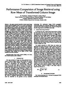
A search length of 4 (k=4) was used, that is, up to 4 images were retrieved in each search. For each image in the data base, the distances of its FV to all other FVs were calculated and the distances ranked. The four images having the smaller distances (considering their FVs) to the query image were retrieved. The value considered in the graph was the average of the values found. 5 Results For the first image data base (generic subjects), all three methods obtained 100% of true answers. This result can be explained observing that all the methods are not sensitive to translation. As reflecting the images in vertical or horizontal directions involves only translation, all the images of the same class will have, in each method, exactly the same FV. Therefore the distances of the FVs of the images in the same class will always be zero and for this reason we have 100% of correct answers. For the second image data base, the three methods had different behavior, as shown in Figure 5. The best performance was obtained when color autocorrelograms were used to generate the FVs, but, surprisingly, the performance of the mixturegram, that considers only 8 colors, was very close to the performance of the autocorrelogram that uses 75 colors. Although the use of perceptual color histograms has presented an inferior performance when compared to the other two methods, the performance is still very good, considering that only 11 colors are used. 6 Conclusions We conclude that the proposed approaches using autocorrelograms, mixturegrams or perceptual color histograms for color quantization are efficient methods for CBIR. Autocorrelograms showed an outstanding performance due to several reasons. It can capture the spatial correlation of colors in an image and therefore excels histograms when used as FVs. Furthermore, the use of HSV color space to quantize the images before generating the autocorrelograms, gives them an additional property of low sensitiveness to illumination changes that occur to certain parts of the faces when the expression changes. Also, the use of relative distances instead of Euclidian distances between FVs give this method an extra advantage over the other two
5
Figure 5. Precision vs. Recall curves for image data base of faces because this distance takes into account not only the absolute difference between FVs, but also considers the sum of the FVs, what can further increase the power of distinction between two different images. Another important point to consider is that the higher number of colors used by the autocorrelogram method makes it easier to distinguish between two different images, what can, in part, explain the superior performance obtained. On the other hand, the small number of colors used by the mixturegram and the perceptual color histogram promote a reduction in the execution time and a drastic reduction on the feature vector sizes, minimizing the “dimensionality” of the FVs with a small loss of performance. Another striking result is that performance is highly dependent on the nature of the images. When the first data base was used, all the methods led to a 100% of correct answers. For the second data base, the performance showed a decrease in performance due to its different nature of the images. Additionally, depending on the nature of the images in the data base, images of a different class from the one being searched can have FVs with smaller distances than the FVs of the images in the class being searched. Concerning the method using perceptual color histograms, its loss in performance can partially be attributed to the way color quantization is carried out. The strong subjective component of this process can result in colors of very different hues being classified as the same perceptual color, what can, in the end, significantly reduce the ability of this method to distinguish between images of different classes. References 1. HUANG, J. et al. (1997). Image indexing using color correlograms. Proc. IEEE Computer Society Conference on Computer Vision and Pattern Recognition, San Juan, Puerto Rico, p. 762-768. 2. Gonzales, R. C., Woods, R. E., and Eddins, Steven L. (2004) Digital Image processing using Matlab. Pearson Education. 3. Evans, R. M. (1948). An Introduction to Color. New York: Wiley. 4. Goldstein, E. B. (1989). Sensation and Perception. 3.ed. California: Wadsworth Publishing Company. 5. Berlin, B.; KaY, P. (1991). Basic Color Terms. California: Berkeley. 6. King, P. J.; Mandani, E. H. (1977). The application of fuzzy control systems to industrial process. Automática. p.235-242.
6