Performance comparison of machine learning techniques in ... - PeerJ

Performance comparison of machine learning techniques in sleep scoring based on wavelet features and neighboring component analysis Behrouz Alizadeh Savareh

1

, Azadeh Bashiri

2

, Ali Behmanesh

3

, Gholam Hossein Meftahi

4

, Boshra Hatef Corresp.

4

1 2 3 4

Student Research Committee, School of Allied Medical Sciences, Shahid Beheshti University of Medical Scinces, Tehran, Iran Health Information Management Department, School of Allied Medical Sciences, Tehran University of Medical Sciences, Tehran, Iran Student Research Committee, School of Health Management and Information Sciences Branch, Iran University of Medical Sciences, Tehran, Iran Neuroscience Research Center, Baqiyatallah University of Medical Sciences, Tehran, Iran

Corresponding Author: Boshra Hatef Email address: [email protected]

Introduction: Sleep scoring is an important step in the treatment of sleep disorders. Manual annotation of sleep stages is time-consuming and experience-relevant and, therefore, needs to be done using machine learning techniques. methods: Sleep-edf polysomnography was used in this study as a dataset. Support Vector Machines and Artificial Neural Network performance were compared in sleep scoring using wavelet tree features and neighborhood component analysis. Results: Neighboring component analysis as a combination of linear and non-linear feature selection method had a substantial role in feature dimension reduction. Artificial neural network and support vector machine achieved 90.30% and 89.93% accuracy respectively. Discussion and Conclusion: Similar to the state of the art performance, introduced method in the present study achieved an acceptable performance in sleep scoring. Furthermore, its performance can be enhanced using a technique combined with other techniques in feature generation and dimension reduction. It is hoped that, in the future, intelligent techniques can be used in the process of diagnosing and treating sleep disorders.

PeerJ Preprints | https://doi.org/10.7287/peerj.preprints.27020v1 | CC BY 4.0 Open Access | rec: 3 Jul 2018, publ: 3 Jul 2018

1

Title:

2 3

Performance comparison of machine learning techniques in sleep scoring based on wavelet features and neighborhood component analysis

4 5 6

Abstract

7

Introduction:

8 9 10

Sleep scoring can be considered as an important step in the treatment of sleep disorders. However, annotating sleep stages manually is time-consuming and requires experience; therefore, it is preferable to perform it using machine learning techniques.

11

Methods:

12 13 14

A sleep-EDF polysomnography dataset was used in this study. The performances of support vector machine (SVM) and artificial neural network (ANN) in sleep scoring were compared using wavelet tree features and neighborhood component analysis.

15

Results:

16 17 18

Neighboring component analysis as a combination of linear and nonlinear feature selection methods had substantially reduced the feature dimensions. ANN and SVM achieved 90.30% and 89.93% accuracy, respectively.

19

Discussion and Conclusion:

20 21 22 23 24

Similar to the state-of-the-art method, the method introduced in the present study achieved an acceptable performance in sleep scoring. Furthermore, its performance could be enhanced by combining it with other techniques for feature generation and dimension reduction. It is expected that in the future, intelligent techniques can be used for diagnosing and treating sleep disorders.

25

Lay Abstract

26 27 28 29

Because sleep scoring by manual method is time-consuming, it is preferable to use machine learning techniques. In this study, a comparison between artificial neural network and support vector machine, based on wavelet features, demonstrated acceptable accuracy in sleep scoring.

30


31

Introduction

32 33 34 35 36

Sleep is a behavioral state characterized by the lack of interaction between an individual and the environment as well as a relative motor quiescence (1). It is worth mentioning that the undeniable impact that sleep has on various human physical and mental activities make it a significant factor in human health (2–5). Thus, it is clear that sleep disorders could lead to devastating effects on various aspects of human life (6).

37 38 39 40 41 42 43 44 45

Regarding the treatment of sleep disorders, polysomnography (PSG) can be considered as the main tool for collecting as well as measuring the electrophysiological signals to analyze body functions during sleep (7). Therefore, an important step here would be hypnogram analysis. A hypnogram is defined as a diagram for identifying the sleep transition between different stages. These stages can be determined based on Rachtschaffen and Kales as wake, sleep with rapid eye movement (REM), non-REM stage 1 (NREM1), stage 2 (NREM2), stage 3 (NREM3), and stage 4 (NREM4) (8). The hypnogram is generated from PSG signals in a period of 20 or 30 s epochs (9) as follows:

46 47



48 49 50 51



52 53 54



55 56



57 58



59 60 61



Wake, comprising over half of the epoch, consists of alpha waves or low voltage, mixed-frequency (2–7 Hz) activity. Stage 1, comprising half of the epoch, consists of relatively low voltage, mixedfrequency (2–7 Hz) activity. At this stage, < 50% of the epoch contains alpha activity. Slow rolling eye movements, lasting several seconds, can be often observed in early Stage 1. Stage 2 occurs with the appearance of sleep spindles and/or K complexes. Moreover, < 20% of the epoch may contain high voltage (75 µV, < 2 Hz) activity. Each sleep spindle and K complex have to last > 0.5 s. Stage 3, comprising 20%–50% of the epoch, consists of high voltage (> 75 µV) and low-frequency (< 2 Hz) activity. Stage 4, comprising over 50% of the epoch, consists of high voltage (> 75 µV, < 2 Hz) and delta activity. REM stage has a relatively low voltage that consists of mixed-frequency (2–7 Hz) electroencephalographic (EEG) activity with episodic REMs and absent or reduced chin electromyographic (EMG) activity (10).

62 63 64 65

However, the main challenge in hypnogram analysis is the recognition of sleep stages, which is very time-consuming and more importantly, depends on the analyst’s individual experience (12 ,11). Hence, computerization of this process would be extremely helpful in saving time and significantly enhancing the accuracy of sleep disorder diagnosis (13).

66 67

Many examples can be mentioned here regarding the application of intelligent techniques in medical diagnostic automation (14–20) and EEG analysis (21–35). In


68 69 70 71 72 73 74 75 76 77 78 79 80 81 82 83

2011, Kravoska et al. achieved 81% accuracy in sleep scoring using various features derived from PSG signals. In their work, they adopted a multidimensional analysis involving quadratic discriminant analysis. It was applied as a classifier using signalspecific features in different frequency bands (36). Furthermore, in 2011, Kuo et al. used features based on multiscale permutation entropy in sleep scoring and achieved 89.1% sensitivity and over 70% accuracy in sleep scoring (37). In another research by Yang et al. (38), multiple structures of artificial neural networks (ANNs) were applied based on energy-specific features from the signals. The obtained results indicated accuracies of 81.1%, 81.7%, and 87.2% for a feed-forward neural network, probabilistic neural network, and recurrent neural network, respectively. In 2016 (20), a combination of methods, based on complete ensemble empirical mode decomposition with adaptive noise (CEEMDAN) and bootstrap aggregating (bagging), was applied on PhysioNet data, which achieved 90.69% accuracy. In 2016, Hassan et al. worked on a single EEG for sleep scoring using normal inverse Gaussian parameters and achieved 90.01% accuracy (31). Their other remarkable accomplishment was the achievement of 93.69% accuracy, which was obtained by using a tunable Q-wavelet transform (32).

84 85 86 87 88 89 90 91 92

PSG analysis requires an optimal method for signal feature extraction. In this regard, wavelet tree decomposition can be particularly useful in extracting meaningful information from PSG signals for sleep scoring. Given the large amount of information generated by the wavelet tree analysis, it is necessary to reduce the dimension of data in a desirable way to make them usable for sleep scoring. In the present study, we introduced a step-by-step method for feature extraction using the wavelet tree analysis and dimensionality reduction using neighborhood component analysis (NCA). Moreover, we made a comparison between two well-known classifiers in sleep scoring, i.e., ANN and SVM.

93


94

Methods

95 96 97 98 99

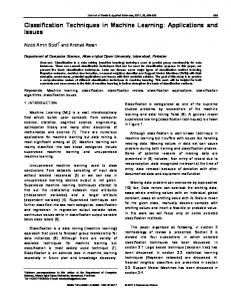
In order to compare these two classifiers based on wavelet features in sleep scoring, a sequential method was proposed in which the following steps were performed: dataset generation, preprocessing, feature extraction, dimensionality reduction, and classification, as shown in Fig. 1. All the steps were implemented using MATLAB 2016b.

100 101 102 103 104

Figure 1. Flowchart of the proposed method for sleep scoring


105

Data

106 107 108 109 110 111 112 113 114

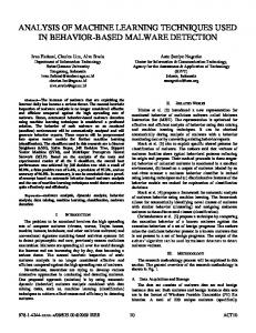
The full version of sleep-EDF from PhysioNet, which is a collection of PSG recordings along with their annotated hypnograms, was used in this study as the initial dataset. The collection of 61 whole-night polysomnographic sleep recordings contained EEG signals of the Fpz-Cz and Pz-Oz channels, electrooculography (EOG) (horizontal), and submental chin EMG signals (Fig. 2) (39). The EOG and EEG signals were sampled at 100 Hz. The submental EMG signal was electronically high-pass filtered, rectified, and low-pass filtered. Then, it was expressed in uV root-mean-square (rms) and sampled at 1 Hz (40). In this dataset, hypnograms were generated for every 30 s of EEG data in accordance with the R&K criteria by well-trained experts (28).

115 116 117

Figure 2. Sample signals from sleep-EDF

118 119 120 121 122 123 124 125 126 127 128 129 130 131

A class-imbalanced dataset is one in which each class of the given dataset is not evenly distributed (41). Notably, an imbalanced dataset is a serious problem in machine learning and data mining (42). Because the number of sleep stages in the dataset was not equal (Table 1), 2000 epochs were randomly selected from each sleep stage (Wake, REM, NREM1, NREM2, NREM3, and NREM4) and a 10,000-sample dataset was generated. It was actually done for the purpose of overcoming the imbalanced situation in the sleep-EDF dataset and reducing the next step’s computations. Although balancing the data can make a slight difference between the actual dataset and the new version, it does not make much sense as the number of samples was relatively high. In addition, balancing the dataset was necessary for classifier training in order to avoid biased learning. Table 1. Stage count in sleep-EDF dataset

132 133

Preprocessing

134 135 136 137 138

In order to remove the noises from the signals, standard deviation normalization was applied as in Eq. 1. Actually, owing to the use of wavelet analysis in the next steps of the study, only standard deviation normalization was used to eliminate the noise in the first step. Further analysis of the noise reduction would be performed later using the wavelet transform.

139 140

𝑋𝑛𝑒𝑤 =

𝑋𝑜𝑙𝑑 ‒ 𝑀𝑒𝑎𝑛 𝑆𝑡𝑑.𝑑𝑒𝑣

Eq. 1. Standard deviation normalization


141 142 143 144

This stage of preprocessing was performed to normalize the signals. Most of the noises were eliminated by multistage wavelet breakdown, owing to the use of the wavelet transform in the next step to extract the features.

145 146

Feature Extraction

147 148 149 150 151 152 153 154 155 156 157

Considering the advancement of the wavelet transformation in analyzing non-stationary signals such as EEG, EOG, and EMG, the wavelet tree analysis was used for feature extraction in this step. Various features were generated based on the wavelet tree analysis (43, 44), which were used as the base features for sleep scoring. According to the wavelet feature extraction and the activity bands of input signals, a tree of wavelet decomposition was applied on signals at each level, and a group of features was generated (Fig. 3). Because it works based on multiresolution approximation by decomposing the signal into a lower resolution space (Aj) and details (Dj), the approximation space (low-frequency band) and detail space (high-frequency band) were frequently decomposed from the previous levels. This recursive splitting of vector space is represented by an admissible wavelet packet tree (45). Energy was calculated using Eq. 2 for each subband of the signal.

158

log (𝑆(𝑙)) = log

∞

(∑ ) 𝑚=1

𝑊𝑥(𝑙,𝑚)2 𝑁𝑙

159

Wx is the wavelet packet transform of signal

160

l is the subband frequency index

161

Ni is the number of wavelet coefficients in the lth subband.

162 163

Eq. 2. Energy calculation of signals (46)

164 165 166 167

Figure 3. Wavelet packet feature extraction from input signal

168 169 170


171 172

Feature Selection

173 174 175 176 177 178 179

Machine learning techniques require a suitable number of inputs to predict intended outputs in the most excellent way. Using a large number of inputs could affect the accuracy and lead to poor performance in many cases. This phenomenon is known as the curse of dimensionality, where increasing the number of features cannot guarantee performance improvement and may even lead to performance decay. Therefore, that phenomenon should be avoided as much as possible to maintain the classifier performance at a satisfactory level (47, 48).

180 181 182 183 184 185 186 187 188 189 190 191 192 193

In the present study, NCA was conducted to avoid the curse of dimensionality. In this technique, the importance of each input is calculated in the output prediction. Then, the important inputs are preserved for the next steps such as classification, fitting, and time series analysis. NCA learns a feature weighting vector by maximizing the expected leave-one-out (LOO) classification accuracy. NCA is a non-parametric method for selecting features with the goal of maximizing the prediction accuracy of the regression and classification algorithms (49). Ideally, this algorithm aims to optimize the classifier performance in the future test data. However, because the real data distribution is not known, the algorithm attempts to optimize the performance based on the training data using the LOO mechanism. The algorithm is restricted to learning Mahalanobis (quadratic) distance metrics. It can always be represented by symmetric positive semidefinite matrices and it can estimate such metrics through its inverse square roots by learning a linear transform of the input space. If it is denoted by a transformation matrix A, a metric is effectively learned as Q = A > A in Eq. 3.

194

𝑑(𝑥, 𝑦) = (𝑥 ‒ 𝑦) > 𝑄(𝑥 ‒ 𝑦) = (𝐴𝑥 ‒ 𝐴𝑦) > (𝐴𝑥 ‒ 𝐴𝑦)

195

Eq. 3. Q matrix calculation in NCA algorithm

196 197 198

The goal of this algorithm is to maximize f(A), which is defined by Eq. 4, using a gradient-based optimizer such as delta-bar-delta or conjugate gradients.

199 200

201 202 203 204

𝑓(𝐴) =

∑ ∑ 𝑝𝑖𝑗 = ∑𝑝𝑖 𝑖 𝑗 ∈ 𝐶𝑖

𝑖

Eq. 4. f(A): class separability as NCA maximization goal

Because the cost function is not convex, some caution must be taken to avoid local maxima during training. Given the fact that its projection is linear, using a nonlinear


205 206 207

classification is recommended in the core of the algorithm to avoid getting stuck in local maxima. This can be attained by using ANN and SVM, which are two well-known classifiers in machine learning techniques.

208 209

Classification

210 211 212 213 214

A review of the literature shows that ANN and SVM have been used in other applications demonstrating the general acceptance of these techniques in different applications of classification tasks (50, 51). Therefore, in the present study, ANN and SVM, as the most popular and successful (52) methods of machine learning, were also selected for sleep scoring.

215 216

Artificial Neural Network

217 218 219 220 221 222 223 224 225 226 227 228

ANN, as a simple simulation of the human brain, tries to imitate the brain learning process using layers of processing units called perceptrons (54 ,53). A single perceptron, as the simplest feed-forward ANN unit, is only capable of learning a linear bi-class separation problem (55-57). However, when a number of perceptrons are combined with each other in the layered structure, they emerge as a powerful mechanism with nonlinear separability, called multilayer perceptron, which is the most famous form of ANNs (Fig. 4). In this regard, ANN is considered as a logical structure with multiprocessing elements, which are connected through interlayer weights. The knowledge of ANN is presented through the weights adjusted during the learning steps. ANN is particularly valuable in processing situations where there is no linear or simple relation between inputs and outputs (58) and in handling unstructured problems with data having no specific distribution models (59).

229 230 231 232

Figure 4. Sample of ANN with one input layer, two hidden layers, and one output layer

233 234 235

The main goal of ANN training is to reduce the error (E) of the classification as Eq. 5:

236


m

𝐸=

237

i=1

n

∑ (yij ‒ yij ∗ )2

j=1

Eq. 5. Error in ANN training phase

238 239 240 241

∑

1 2

In Eq. 5, yij and yij* are the actual and network outputs of the jth output from ith input vector respectively. In order to train and test the ANN structures, ANN models are implemented using the settings in Table 2.

242 243

Table 2. ANN model setting in Matlab

244 245

Support Vector Machine

246 247 248 249 250 251 252 253

SVM has become popular owing to its significantly better empirical performance compared with other techniques (60). SVM, with a strong mathematical basis, is closely related to some well-established theories in statistics and is capable of nonlinear separation using the hyperplane idea. It tries not only to correctly classify the training data, but also to maximize the margin for better generalization of the forthcoming data (61). Its formulation leads to a separating hyperplane that depends only on the small fraction of data points lying on the classification margins, called support vectors (bold texts in Fig. 5).

254 255 256 257

Figure 5. Support vector in SVM


259 260 261 262 263 264 265 266 267

In SVM training phase, tuning of the parameters involves choosing the kernel function and the box constraint (C). The box constraint is a tradeoff parameter between regularization and accuracy, which influences the behavior of support vector selection (62). The kernel, as a key part of the SVM, is a function for transmitting information from the current space to a new hyperspace (63). Because the Gaussian radial-basis function (RBF) kernel is popular, and RBF kernels are shown to perform better than linear or polynomial kernels (64), the RBF function was selected in this study as the kernel for the SVM classifier. The RBF kernel is defined as Eq. 6, where σ is the most important factor to control the RBF kernel in transmitting data to a new hyperspace. '

(

𝐾(𝑥,𝑥 ) = exp ‒

268

‖𝑥 ‒ 𝑥'‖2 2𝜎2

)

269

Eq. 6. RBF kernel

270 271 272 273

As mentioned earlier, to achieve the optimal performance, two parameters of SVM (box constraint (C) and RBF sigma (S)) are important and should be tuned as correctly as possible. To tune these parameters, two cycles are defined in terms of accuracy for exploring the values (Table 3) and choosing the best model with the highest accuracy.

274 275

Table 3. Parameter tuning

276

Validation of Models

277 278 279 280 281 282 283 284

Validation of the results was performed in a different mode for each model. Intermittent ‘‘validation” was performed for ANN during training to avoid over-training problems. In this type of validation, the network is periodically validated with a different dataset. This process is repeated until the validation error begins to increase. At this point, ANN training is terminated, and the ANN is then tested with a third dataset to evaluate how effectively it has learned the generalized behavior (65). In this method, while training the network, as previously mentioned, 70% of the data were used to train the ANN whereas 15% were used for testing and 15% for validation purposes.

285 286 287 288 289 290 291 292 293

For the support vector, the cross-validation method was used to validate the modeling and testing. Cross-validation is a statistical method for evaluating and comparing learning algorithms. It is performed by dividing the data into two segments: one for learning or training the model and the other for validating the model. In a typical crossvalidation, the training and validation sets must cross over in the successive rounds such that each data point has a chance of being validated. The basic form of crossvalidation is K-fold cross-validation (66), which randomly divides the original sample into K subsamples. Then, a single subsample is selected as the validation data for testing the model, and the remaining K-1 subsamples are used as the training data.


294 295 296 297 298

This process is repeated K times, and each K subsample is used exactly once as the validation data. The K results from the folds can then be averaged (or otherwise combined) to produce a single estimation (67). This strategy was used for SVM validation using K = 10 and the mean accuracy was considered as the final accuracy for SVM.

299 300

Result

301 302 303 304 305 306

Based on the activity bands of the input signals, six levels of wavelet tree feature extraction were used and a total number of approximately 3500 features were generated for PSG signals in each epoch. As the large number of features can greatly increase the risk of the curse of dimensionality, the NCA algorithm was used for feature selection (to avoid the mentioned risk).

307 308 309 310 311

To reduce the dimensions of the data using the NCA algorithm and to select the features, a threshold level of 0.1 was determined for weight screening. This value was selected by examining the appropriate number of output parameters based on threshold levels, where the goal of this step was to reduce the number of dimensions to 37. Figure 6 shows the NCA value (y-axis) for the selected features (x-axis) in a descending order.

312 313 314 315 316 317 318 319

Figure 6. NCA output values for 37 selected features from wavelet tree analysis As a rule of thumb, in the classification phase, all architectures with one or two hidden layers were investigated to achieve the best architecture in the ANN design. In each layer, as many neurons as one to three times the number of inputs were explored (Fig. 7).

320 321 322 323

Figure 7. Results of different ANN structures

324 325 326

Figure 7 shows the accuracy values for different layering modes of the ANN, where the horizontal axis is the number of neurons in the first hidden layer and the vertical one is the number of neurons in the second hidden layer. Based on the results, an architecture


327 328 329

with one input layer (37 neurons = number of selected features), two hidden layers (75 neurons, 76 neurons), and one output layer (with 5 neurons = the number of sleep stages) was considered as the optimal architecture (Fig. 8).

330 331 332 333 334 335 336 337 338

Figure 8. ANN architecture for sleep scoring According to the information theory, if the target and predicted outputs of the ANN represent two probable distributions, their cross-entropy is a natural measure of their difference (68). It should be noted that cross-entropy is an appropriate criterion for assessing the training and controlling the ANN, if necessary. Figure 9 shows the crossentropy values over epochs for network training.

339 340 341 342 343

Figure 9. Network training cross-entropy

344 345 346 347 348 349 350 351 352 353 354

For the five-class sleep scoring, ANN achieved a 90.3% accuracy, which is near the performance of the state-of-the-art method. As another assessment, the receiver operating characteristic (ROC) can be used as a statistic for the predictive test in a binary classification task. The ROC curve is a graphic representation of the sensitivity and specificity of the test across the entire range of the possible classification cut-offs. A 0.50 area under the ROC curve indicates a random test performance, whereas 1.00 is considered as perfect (69). Actually, these charts demonstrate the classifier’s ability to separate each class from the others. Converting the five-class classification problem into five binary classifications (each class versus the other classes) provides a benchmark for analyzing the classifier’s performance. Figure 10 shows the network performance on the test data section in the ROC curve.

355 356 357 358 359

Figure 10. ANN ROC In SVM training, various values were generated and tested as SVM parameters (box constraint and RBF sigma), and the accuracy was evaluated in each situation. The


360 361

result of this step led to the creation of a chart of accuracy based on the parameters (Fig. 11).

362 363 364 365

Figure 4. SVM accuracy based on various box constraints and RBF sigma

366 367 368 369

Based on the optimal parameters, the SVM model was created using the training samples, and a test was carried out based on the test samples. The SVM performance was evaluated as 89.93% in mean accuracy. Figure 12 shows the ROC diagram for SVM in a five-class sleep scoring with Area under the curve (AUC) = 0.91.

370 371

Figure 12. SVM ROC

372 373 374 375

Furthermore, Fig. 13 shows a comparison of the performance of both ANN and SVM versus the state-of-the-art methods. As shown in the figure, the method introduced in this study achieved almost the same performance as that of the state of the art.

376 377 378

Figure 5. Accuracy comparison

379 380 381 382 383 384 385 386 387 388 389

As stated in (70), applying some primary criteria is important for evaluating the algorithms based on the validity of the reports. In the present study, the mentioned criteria were used as widely as possible in data preparation, data splitting, training the model, and reporting; however, each study, based on its intended purpose, examines a certain aspect of efficiency. Regarding the classification of sleep stages, choosing the accuracy as the main parameter of performance evaluation is an appropriate choice and has been considered in most sleep scoring studies. It should be noted that the cost of achieving the optimal performance was also examined for both ANN and SVM techniques. Given the different layers and nodes, the ANN training took a total of approximately 8 h on Intel Core i7 3 GHz laptop with 8 GB RAM, whereas checking different parameters of SVM took approximately 1 h on the same device.

390 391

Discussion and Conclusion


392 393 394 395 396

The analysis of the studies on automatic sleep scoring reveals that the number of these studies is increasing in recent years (28–35). Moreover, the comparison of previous methods of sleep scoring with the introduced method in the present study showed some interesting points. In general, it can be concluded that the three phases including feature extraction, selection, and classification have been used in most of the studies.

397 398 399 400 401 402

In terms of features extracted from signals in the previous methods of sleep scoring, there were various techniques including spectral measures (32), nonlinear measures (71), multiscale entropy (72), energy features from frequency bands (38), and empirical mode decompositions (20). Moreover, features from dual tree complex wavelet transform, tunable Q-factor wavelet transform (32), normal inverse Gaussian pdf modeling (31), and statistical moments (35) were used in the feature extraction phase.

403 404 405

The common property of these methods is the analysis of signal information at different times and frequency resolutions, which provide a detailed information of the signal at different levels.

406 407 408 409 410 411

Of course, the nature of biological signals, particularly those related to the brain function, show non-stationary properties and therefore, requires a combined timefrequency analysis simultaneously. It should be noted that, the advantage of the method used in this study is the capability to perform simultaneous time-frequency analysis of the signals with high precision, and to finally present them in the form of energy parameters.

412 413 414 415 416

Energy extraction with the help of the multispectral analysis is valuable in the analysis of PSG signals. However, the volume of generated information is very high and each epoch of the PSG signals is mapped to a new sample in a space with a very high dimensionality. Therefore, it is necessary to control the huge amount of generated information to prevent the curse of dimensionality risk in the sleep scoring process.

417 418 419 420 421 422 423 424 425 426 427

In this regard, various methods have been used to reduce the dimension including manual selection of features, using transforms such as Quadratic and Linear discriminant analysis, and statistical analysis. In the present study, NCA, which combines linear and nonlinear analysis simultaneously, was used to reduce the number of dimensions. It decreases the dimensions based on a combination of linear and nonlinear operations in a mixed mode. According to the results from NCA, this method reduced the initial number of features generated by the wavelet tree analysis to 37 with a compression rate of approximately 0.01. In addition to the quantitative power of the method in compressing the feature dimensions, the selected features had also a good quality when they were used at the next stage as the input of the classifiers, leading to an acceptable performance.

428 429

Surveying studies have applied various classifier techniques such as QDA, LDA, ANNs, boosted decision tree, random forest, bagging (ANN), and adaptive boosting in sleep


430 431 432 433 434 435 436 437 438 439 440 441

scoring. In this study, ANN and SVM were used for testing sleep scoring based on the features generated by the wavelet tree analysis. The features were then compressed using the NCA algorithm. One of the most successful studies in automatic sleep scoring applied CEEMDAN with bootstrap aggregating (bagging with a decision tree core) and achieved a 90.69% accuracy in sleep scoring (28). Another study applied tunable Qwavelet transform features with various spectral features and achieved an overall accuracy of 91.50% for a five-class sleep scoring (32). Moreover, another study achieved 93.69% accuracy using a decomposed two-subband tunable Q wavelet transform and four statistical moments extracted for each subband (35). In terms of overall accuracy (five-class separation), applying our methods on the sleep-EDF dataset achieved 90.33% and 89.93% accuracies for ANN and SVM respectively, which are close to the performance of the state of the art (see Table 4 to Table 7).

442

Table 4. ANN confusion matrix

443 444

Table 5. ANN evaluation metrics

445 446

Table 6. SVM confusion matrix

447 448

Table 7. SVM evaluation metrics

449 450 451 452 453 454 455 456 457 458 459 460 461 462 463

In the end, the following are the points worth mentioning. In the present study, the wavelet tree analysis was used for feature extraction from biological signals both in the time and frequency domains, because of its ability to mine very precise information about the signal energy. Notably, the wavelet tree produced high-dimensional features, which should be handled using a suitable method. In this regard, the NCA, as a combination of linear and nonlinear methods, was used to compress the information in an excellent way, both quantitatively and qualitatively. Thus, the advantage of this study was the use of the NCA method in reducing the dimensions of features appropriately by the simultaneous analysis of both linear and nonlinear features (although some similar studies had also achieved a good performance using some other classifiers). Given the modular capability of the method presented in this study, it is possible to replace any of its elements in the feature extraction, feature compression, and classification. Therefore, future studies can be directed toward changing each element to achieve better performance.

464


465

Limitations

466 467

This study was limited to the acquisition of local sleep EEG datasets. Accessing such dataset could help validate its results more accurately.

468


469

References:

470 471 472 473 474 475 476 477 478 479 480 481 482 483 484 485 486 487 488 489 490 491 492 493 494 495 496 497 498 499 500 501 502 503 504 505 506 507 508 509 510 511 512 513 514 515

1. Nofzinger EA, Mintun MA, Wiseman M, Kupfer DJ, Moore RY. Forebrain activation in REM sleep: an FDG PET study. Brain research. 1997;770(1):192-201. 2. Hays RD, Stewart A. Sleep measures. 1992. 3. Czeisler CA, Klerman EB. Circadian and sleep-dependent regulation of hormone release in humans. Recent progress in hormone research. 1999;54:97-130; discussion -2. 4. Tibbitts GM. Sleep disorders: causes, effects, and solutions. Primary Care: Clinics in Office Practice. 2008;35(4):817-37. 5. Tavallaie S, Assari S, Najafi M, Habibi M, Ghanei M. Study of sleep quality in chemical-warfareagents exposed veterans. Journal Mil Med. 2005;6(4):241-8. 6. Buysse DJ, Grunstein R, Horne J, Lavie P. Can an improvement in sleep positively impact on health? Sleep Medicine Reviews. 2010;14(6):405-10. 7. Nofzinger EA. Neuroimaging and sleep medicine. elsevier. 2005(Sleep Medicine Reviews):15772. 8. Merica H, Fortune RD. State transitions between wake and sleep, and within the ultradian cycle, with focus on the link to neuronal activity. Sleep Medicine Reviews. 2004;8(6):473-85. 9. Rossow AB, Salles EOT, Co, x, co KF, editors. Automatic sleep staging using a single-channel EEG modeling by Kalman Filter and HMM. Biosignals and Biorobotics Conference (BRC), 2011 ISSNIP; 2011 68 Jan. 2011. 10. Maeda M, Takajyo A, Inoue K, Kumamaru K, Matsuoka S, editors. Time-frequency analysis of human sleep EEG and its application to feature extraction about biological rhythm. SICE, 2007 Annual Conference; 2007: IEEE. 11. Ronzhina M, Janousek O, Kolárová J, Nováková M, Honzík P, Provazník I. Sleep scoring using artificial neural networks. Elsevier. 2011. 12. Gath I, Bar-On E. Computerized method for scoring of polygraphic sleep recordings. Computer Programs in Biomedicine. 1980;11(3):217-23. 13. Innocent PR, John RI, Garibaldi JM. Fuzzy methods and medical diagnosis. 2004. 14. Hassan AR, Haque MA. Computer-aided gastrointestinal hemorrhage detection in wireless capsule endoscopy videos. Computer Methods and Programs in Biomedicine. 2015;122(3):341-53. 15. Bashar SK, Hassan AR, Bhuiyan MIH, editors. Identification of motor imagery movements from eeg signals using dual tree complex wavelet transform. Advances in Computing, Communications and Informatics (ICACCI), 2015 International Conference on; 2015: IEEE. 16. Hassan AR. Computer-aided obstructive sleep apnea detection using normal inverse Gaussian parameters and adaptive boosting. Biomedical Signal Processing and Control. 2016;29:22-30. 17. Hassan AR, Haque MA. Computer-aided obstructive sleep apnea screening from single-lead electrocardiogram using statistical and spectral features and bootstrap aggregating. Biocybernetics and Biomedical Engineering. 2016;36(1):256-66. 18. Hassan AR, editor Automatic screening of obstructive sleep apnea from single-lead electrocardiogram. Electrical engineering and information communication technology (ICEEICT), 2015 international conference on; 2015: IEEE. 19. Hassan AR, editor A comparative study of various classifiers for automated sleep apnea screening based on single-lead electrocardiogram. Electrical & Electronic Engineering (ICEEE), 2015 International Conference on; 2015: IEEE. 20. Hassan AR, Haque MA, editors. Identification of Sleep Apnea from Single-Lead Electrocardiogram. Computational Science and Engineering (CSE) and IEEE Intl Conference on Embedded and Ubiquitous Computing (EUC) and 15th Intl Symposium on Distributed Computing and Applications for Business Engineering (DCABES), 2016 IEEE Intl Conference on; 2016: IEEE.


516 517 518 519 520 521 522 523 524 525 526 527 528 529 530 531 532 533 534 535 536 537 538 539 540 541 542 543 544 545 546 547 548 549 550 551 552 553 554 555 556 557 558 559 560 561 562 563

21. Hassan AR, Haque MA. An expert system for automated identification of obstructive sleep apnea from single-lead ECG using random under sampling boosting. Neurocomputing. 2017;235:122-30. 22. Bashar SK, Hassan AR, Bhuiyan MIH, editors. Motor imagery movements classification using multivariate emd and short time fourier transform. India Conference (INDICON), 2015 Annual IEEE; 2015: IEEE. 23. Hassan AR, Haque MA, editors. Computer-aided sleep apnea diagnosis from single-lead electrocardiogram using dual tree complex wavelet transform and spectral features. Electrical & Electronic Engineering (ICEEE), 2015 International Conference on; 2015: IEEE. 24. Hassan AR, Haque MA. Computer-aided obstructive sleep apnea identification using statistical features in the EMD domain and extreme learning machine. Biomedical Physics & Engineering Express. 2016;2(3):035003. 25. Hassan AR, Siuly S, Zhang Y. Epileptic seizure detection in EEG signals using tunable-Q factor wavelet transform and bootstrap aggregating. Computer methods and programs in biomedicine. 2016;137:247-59. 26. Hassan AR, Subasi A. Automatic identification of epileptic seizures from EEG signals using linear programming boosting. Computer methods and programs in biomedicine. 2016;136:65-77. 27. Hassan AR, Haque MA, editors. Epilepsy and seizure detection using statistical features in the complete ensemble empirical mode decomposition domain. TENCON 2015-2015 IEEE Region 10 Conference; 2015: IEEE. 28. Hassan AR, Bhuiyan MIH. Computer-aided sleep staging using complete ensemble empirical mode decomposition with adaptive noise and bootstrap aggregating. Biomedical Signal Processing and Control. 2016;24:1-10. 29. Hassan AR, Bhuiyan MIH. Automatic sleep scoring using statistical features in the EMD domain and ensemble methods. Biocybernetics and Biomedical Engineering. 2016;36(1):248-55. 30. Hassan AR, Bhuiyan MIH, editors. Dual tree complex wavelet transform for sleep state identification from single channel electroencephalogram. Telecommunications and Photonics (ICTP), 2015 IEEE International Conference on; 2015: IEEE. 31. Hassan AR, Bhuiyan MIH. An automated method for sleep staging from EEG signals using normal inverse Gaussian parameters and adaptive boosting. Neurocomputing. 2017;219:76-87. 32. Hassan AR, Bhuiyan MIH. A decision support system for automatic sleep staging from EEG signals using tunable Q-factor wavelet transform and spectral features. Journal of neuroscience methods. 2016;271:107-18. 33. Hassan AR, Bashar SK, Bhuiyan MIH, editors. On the classification of sleep states by means of statistical and spectral features from single channel electroencephalogram. Advances in Computing, Communications and Informatics (ICACCI), 2015 International Conference on; 2015: IEEE. 34. Hassan AR, Bashar SK, Bhuiyan MIH, editors. Automatic classification of sleep stages from singlechannel electroencephalogram. India Conference (INDICON), 2015 Annual IEEE; 2015: IEEE. 35. Hassan AR, Subasi A. A decision support system for automated identification of sleep stages from single-channel EEG signals. Knowledge-Based Systems. 2017;128:115-24. 36. Krakovská A, Mezeiová K. Automatic sleep scoring: A search for an optimal combination of measures. Artificial intelligence in medicine. 2011;53(1):25-33. 37. Kuo C-E, Liang S-F, editors. Automatic stage scoring of single-channel sleep EEG based on multiscale permutation entropy. Biomedical Circuits and Systems Conference (BioCAS), 2011 IEEE; 2011: IEEE. 38. Hsu Y-L, Yang Y-T, Wang J-S, Hsu C-Y. Automatic sleep stage recurrent neural classifier using energy features of EEG signals. Neurocomputing. 2013;104:105-14. 39. Kemp B. The sleep-edf database online. URL http://www physionet org/physiobank/database/sleep-edf. 2013.


564 565 566 567 568 569 570 571 572 573 574 575 576 577 578 579 580 581 582 583 584 585 586 587 588 589 590 591 592 593 594 595 596 597 598 599 600 601 602 603 604 605 606 607 608 609 610 611

40. Kemp B, Zwinderman AH, Tuk B, Kamphuisen HA, Oberye JJ. Analysis of a sleep-dependent neuronal feedback loop: the slow-wave microcontinuity of the EEG. IEEE Transactions on Biomedical Engineering. 2000;47(9):1185-94. 41. Mohd Pozi MS, Sulaiman MN, Mustapha N, Perumal T. A new classification model for a class imbalanced data set using genetic programming and support vector machines: case study for wilt disease classification. Remote Sensing Letters. 2015;6(7):568-77. 42. Al Helal M, Haydar MS, Mostafa SAM, editors. Algorithms efficiency measurement on imbalanced data using geometric mean and cross validation. Computational Intelligence (IWCI), International Workshop on; 2016: IEEE. 43. Khushaba RN, Kodagoda S, Lal S, Dissanayake G. Driver drowsiness classification using fuzzy wavelet-packet-based feature-extraction algorithm. IEEE Transactions on Biomedical Engineering. 2011;58(1):121-31. 44. Savareh BA, Sadat Y, Bashiri A, Shahi M, Davaridolatabadi N. The design and implementation of the software tracking cervical and lumbar vertebrae in spinal fluoroscopy images. Future science OA. 2017;3(4):FSO240. 45. Khushaba RN, Al-Jumaily A. Fuzzy wavelet packet based feature extraction method for multifunction myoelectric control. International Journal of Biomedical Sciences. 2007. 46. Khushaba RN, Al-Jumaily A, Al-Ani A, editors. Novel feature extraction method based on fuzzy entropy and wavelet packet transform for myoelectric Control. Communications and Information Technologies, 2007 ISCIT'07 International Symposium on; 2007: IEEE. 47. Keogh E, Mueen A. Curse of dimensionality. Encyclopedia of Machine Learning: Springer; 2011. p. 257-8. 48. Savareh BA, Ghanjal A, Bashiri A, Motaqi M, Hatef B. The power features of Masseter muscle activity in tension-type and migraine without aura headache during open-close clench cycles. PeerJ. 2017;5:e3556. 49. Yang W, Wang K, Zuo W. Neighborhood Component Feature Selection for High-Dimensional Data. JCP. 2012;7(1):161-8. 50. Liu Z, Cheng K, Li H, Cao G, Wu D, Shi Y. Exploring the potential relationship between indoor air quality and the concentration of airborne culturable fungi: a combined experimental and neural network modeling study. Environmental Science and Pollution Research. 2018;25(4):3510-7. 51. Li H, Liu Z, Liu K, Zhang Z. Predictive Power of Machine Learning for Optimizing Solar Water Heater Performance: The Potential Application of High-Throughput Screening. International Journal of Photoenergy. 2017;2017. 52. Sammut C, Webb GI. Encyclopedia of machine learning: Springer Science & Business Media; 2011. 53. Vaisla KS, Bhatt AK. An analysis of the performance of artificial neural network technique for stock market forecasting. International Journal on Computer Science and Engineering. 2010;2(6):2104-9. 54. Ferreira EC, Milori DM, Ferreira EJ, Da Silva RM, Martin-Neto L. Artificial neural network for Cu quantitative determination in soil using a portable laser induced breakdown spectroscopy system. Spectrochimica Acta Part B: Atomic Spectroscopy. 2008;63(10):1216-20. 55. Pradhan B, Lee S. Landslide susceptibility assessment and factor effect analysis: backpropagation artificial neural networks and their comparison with frequency ratio and bivariate logistic regression modelling. Environmental Modelling & Software. 2010;25(6):747-59. 56. Mohammadfam I, Soltanzadeh A, Moghimbeigi A, Savareh BA. Use of artificial neural networks (ANNs) for the analysis and modeling of factors that affect occupational injuries in large construction industries. Electronic physician. 2015;7(7):1515. 57. Alizadeh B, Safdari R, Zolnoori M, Bashiri A. Developing an intelligent system for diagnosis of asthma based on artificial neural network. Acta Informatica Medica. 2015;23(4):220.


612 613 614 615 616 617 618 619 620 621 622 623 624 625 626 627 628 629 630 631 632 633 634 635 636 637 638 639 640 641 642 643 644

58. Singh SK, Mahesh K, Gupta AK. Prediction of mechanical properties of extra deep drawn steel in blue brittle region using Artificial Neural Network. Materials & Design (1980-2015). 2010;31(5):2288-95. 59. Jani HM, Islam AT, editors. A framework of software requirements quality analysis system using case-based reasoning and Neural Network. Information Science and Service Science and Data Mining (ISSDM), 2012 6th International Conference on New Trends in; 2012: IEEE. 60. Trivedi SK, Dey S. Effect of various kernels and feature selection methods on SVM performance for detecting email spams. International Journal of Computer Applications. 2013;66(21). 61. Ge Z, Gao F, Song Z. Batch process monitoring based on support vector data description method. Journal of Process Control. 2011;21(6):949-59. 62. De Leenheer P, Aabi M. Support Vector Machines: Analyse van het Gedrag & Uitbreiding naar Grootschalige Problemen. 63. Hsu C-W, Chang C-C, Lin C-J. A practical guide to support vector classification. 2003. 64. Bsoul M, Minn H, Tamil L. Apnea MedAssist: real-time sleep apnea monitor using single-lead ECG. IEEE Transactions on Information Technology in Biomedicine. 2011;15(3):416-27. 65. Omid M, Mahmoudi A, Omid MH. Development of pistachio sorting system using principal component analysis (PCA) assisted artificial neural network (ANN) of impact acoustics. Expert Systems with Applications. 2010;37(10):7205-12. 66. Refaeilzadeh P, Tang L, Liu H. Cross-validation. Encyclopedia of database systems: Springer; 2009. p. 532-8. 67. Jiang P, Chen J. Displacement prediction of landslide based on generalized regression neural networks with K-fold cross-validation. Neurocomputing. 2016;198:40-7. 68. Blumstein DT, Bitton A, DaVeiga J. How does the presence of predators influence the persistence of antipredator behavior? Journal of Theoretical Biology. 2006;239(4):460-8. 69. Mattsson N, Rosen E, Hansson O, Andreasen N, Parnetti L, Jonsson M, Herukka SK, Van Der Flier WM, Blankenstein MA, Ewers M, Rich K. Age and diagnostic performance of Alzheimer disease CSF biomarkers. Neurology. 2012 Feb 14;78(7):468-76. 70. Maeda T. how to rationally compare the performances of different machine learning models? PeerJ Preprints, 2018 2167-9843. 71. Akgul T, Mingui S, Sclahassi RJ, Cetin AE. Characterization of sleep spindles using higher order statistics and spectra. Biomedical Engineering, IEEE Transactions on. 2000;47(8):997-1009. 72. Liang S-F, Kuo C-E, Hu Y-H, Pan Y-H, Wang Y-H. Automatic stage scoring of single-channel sleep EEG by using multiscale entropy and autoregressive models. IEEE Transactions on Instrumentation and Measurement. 2012;61(6):1649-57.

645


Figure 1 The flowchart of the proposed method for sleep scoring



Figure 2 PolySomnoGraphy signal values


Figure 3 Wavelet packet feature extraction from input signal


Figure 4 A sample of ANN with one input layer, two hidden layers and one output layer


Figure 5 Support vector in SVM Each point shows a sample of data.


Figure 6 NCA output values


Figure 7 ANN Accuracy values


Figure 8 Artificial Neural Network Architecture for sleep scoring


Figure 9 Network training cross entropy The lines show the network performance: B: Train G: Validation R: Test.


Figure 10 ANN ROC ROC for 5 classes: Blue: Wake Dark Green: N1 Light Green: N2 Red: N3 Purple: REM.


Figure 11 SVM Accuracy values


Figure 12 SVM ROC


Figure 13 Accuracy comparison


Table 1(on next page) Stages count in sleep- edf


1

Table1.Stages count in sleep-edf Stage Count Wake 77327 N1 4664 N2 26560 N3 9049 REM 11618

2


Table 2(on next page) ANNs model setting in Matlab


1 2

Table2. ANNs model setting in Matlab Setting Activation function preprocess function Data partitioning mode Network performance evaluation Iteration

Value Tangent sigmoid Remove constant rows random Cross entropy 1000

3


Table 3(on next page) parameters tuning


1 2

Table3. parameters tuning parameters Gamma range Box Constraint range

Setting Outer product of log space (-1,.1,10) and np.array([1,10])) Outer product of log space (-1, .1, 10) and np.array([1,10])

3


Table 4(on next page) ANN Confusion matrix


1

Table4. ANN Confusion matrix Target

Wake

N1

N2

N3

Rem

Out Wake N1 N2 N3 Rem

305 5 0 0 5

3 256 11 1 22

0 6 252 6 6

1 0 7 277 20

1 8 43 0 265

2


Table 5(on next page) ANN Evaluation metrics


1

Table5. ANN Evaluation metrics Metrics Accuracy Error Sensitivity Specificity Precision False Positive Rate F1_score Matthews Correlation Coefficient Kappa

Values 0.9033 0.0967 0.9057 0.9758 0.9039 0.0242 0.9034 0.8803 0.6979

2


Table 6(on next page) SVM Confusion matrix


Table6. SVM Confusion matrix

1 Target

Wake

N1

N2

N3

Rem

Out Wake N1 N2 N3 Rem

292 2 0 1 1

5 232 5 2 32

0 19 275 8 10

0 3 10 288 0

1 44 7 1 262

2


Table 7(on next page) SVM Evaluation metrics


1

Table7. SVM Evaluation metrics Metrics Accuracy Error Sensitivity Specificity Precision False Positive Rate F1_score Matthews Correlation Coefficient Kappa

Values 0.8993 0.1007 0.8996 0.9748 0.8994 0.0252 0.8991 0.8743 0.6854

2


Performance comparison of machine learning techniques in ... - PeerJ

Performance comparison of machine learning techniques in ... - PeerJ

Suggest Documents

Performance comparison of machine learning

Performance Evaluation of Machine Learning Techniques using ...

Performance Comparison of Learning Techniques for

comparison of machine learning techniques in phishing website ...

A comparison of machine learning techniques for survival prediction in ...

A comparison of machine learning techniques for survival prediction in ...

Classification Techniques in Machine Learning

MLitB: machine learning in the browser - PeerJ

Comparison of Machine Learning Techniques using the ... - IEEE Xplore

A comparison of machine learning techniques for ... - Google Sites

Comparison of machine-learning techniques for handling ... - SC15

Comparison of Machine Learning Techniques with ... - Semantic Scholar

comparison of machine learning techniques for document ranking

A Comparison of Machine Learning Techniques for Modeling Human ...

Comparison of Machine Learning Techniques for Fetal Heart Rate ...

Comparison of Recent Machine Learning Techniques for Gender ...

Comparison of Recent Machine Learning Techniques for Gender ...

A comparison of machine learning techniques for ...

ANALYSIS OF MACHINE LEARNING TECHNIQUES USED IN ...

Application of Machine Learning Techniques in Aquaculture

Using Machine Learning Techniques to Enhance the Performance of ...

Comparison of machine learning and deep learning

Performance comparison of machine learning ... - PeerJwww.researchgate.net › publication › fulltext › Performan

Machine Learning Techniques for Exoplanet