Using Machine Learning Techniques to Enhance the Performance of ...

Using Machine Learning Techniques to Enhance the Performance of an Automatic Backup and Recovery System Dan Pelleg ∗

Eran Raichstein†

ABSTRACT A typical disaster recovery system will have mirrored storage at a site that is geographically separate from the main operational site. In many cases, communication between the local site and the backup repository site is performed over a network which is inherently slow, such as a WAN, or is highly strained, for example due to a whole-site disaster recovery operation. The goal of this work is to alleviate the performance impact of the network in such a scenario, and to do so using machine learning techniques. We focus on two main areas, prefetching and readahead size determination. In both cases we significantly improve the performance of the system. Our main contributions are as follows: We introduce a theoretical model of the system and the problem we are trying to solve and bound the gain from prefetching techniques. We construct two frequent pattern mining algorithms and use them for prefetching. A framework for controlling and combining multiple prefetch algorithms is presented as well. These algorithms, as well as various simple prefetch algorithms, are compared on a simulation environment. We introduce a novel algorithm for determining the amount of read ahead on such a system that is based on intuition from online competitive analysis and on regression techniques. The significant positive impact of this algorithm is demonstrated on IBM’s FastBack system. Much of our improvements have been applied with little or no modification of the current implementation’s internals. We therefore feel confident in stating that the techniques are general and are likely to have applications elsewhere.

Categories and Subject Descriptors D.4.2 [Storage Management]; D.4.5 [Reliability]: Backup procedures; F.2 [ANALYSIS OF ALGORITHMS AND PROBLEM ∗

IBM, Haifa Research Lab, Haifa University Campus, Mount Carmel, Haifa, Israel. Email: [email protected] † IBM Software Group, Building 30, Matam, Haifa, Israel. Email: [email protected] ‡ IBM, Haifa Research Lab, Haifa University Campus, Mount Carmel, Haifa, Israel. Email: [email protected]

Permission to make digital or hard copies of all or part of this work for personal or classroom use is granted without fee provided that copies are not made or distributed for profit or commercial advantage and that copies bear this notice and the full citation on the first page. To copy otherwise, to republish, to post on servers or to redistribute to lists, requires prior specific permission and/or a fee. SYSTOR 2010 May 24-26, Haifa, Israel Copyright 2010 ACM X-XXXXX-XX-X/XX/XX ...$10.00.

Amir Ronen‡

COMPLEXITY]; I.2.6 [Learning]

General Terms Algorithms, Machine learning, Systems

Keywords File and storage systems, Readahead, Prefetching

1. 1.1

INTRODUCTION Motivation

A typical disaster recovery system will have mirrored storage at a site that is geographically separate from the main operational site. In many cases, communication between the local (main) site and the (remote) backup repository site is performed over a WAN. The implication for both local data updates and recovery operations is increased latency and reduced bandwidth. This can severely affect performance, and precisely at a point that is critical to any organization’s business operation - the storage system. This paper explores several methods to alleviate the problem using techniques from machine-learning and online analysis. The first assumption we make is that anything beyond the storage controller cannot be modified. That is, we can modify neither the layout of disk blocks nor the file system, the cache sizes are constant, as is the number of spindles, and the file formats are fixed1 . The second assumption precludes changes to the communication protocol. This black-box approach might seem restrictive at first, but in fact opens the door for applicability in a wide range of products and at different levels of the storage hierarchy. In particular, we base our work and findings on the FastBack™ software. This is a data protection and disaster recovery system that is being successfully sold by IBM for the small medium business market. With the proliferation of remote office installations and the advent of 10Gbit Ethernet and other fast networks, performance — especially restore performance — becomes an important part of this suite. However, improving performance is not an isolated step, and typically requires protocol re-design. This always comes at a significant cost in development, testing, migration of existing repositories to new formats, and increased risk of introducing bugs. By taking the black-box approach as described above, we were able to make significant progress toward the goal, incurring only minimal costs. The success also leads us to believe the same line of thinking is likely generalizable to different problems in various application areas. 1

This precludes de-duplication, which changes the layout of disk blocks. De-duplication has many merits, however it is orthogonal to the work in this paper.

1.2

Description of the system and architecture

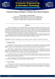
The basic FastBack backup process is block-based with continuous data protection and point-in-time recovery capabilities. It builds on a shim that intercepts disk accesses (e.g. an MS-Windows or Linux disk driver). Modified blocks are sent over the network to a database on a remote server, known as a backup repository. The repository stores the deltas with their corresponding timestamps in a data structure that supports recovery to arbitrary points in the past. The restore process supports two modes: instant restore (IR) and mount. In instant restore, an obliterated disk image is streamed from the repository to the local version in a way that allows the local machine to function normally, well before the image is fully retrieved. Again, a local shim intercepts accesses and traps reads to missing disk blocks. The required block is retrieved from the repository and written to the local disk, at which point the local read request completes. This allows the user, after booting up the system, to start performing useful work within minutes. The full disk recovery process may still take a long time, as dictated by the network speed and data volume, but once the “hot” part of the disk is brought in, the recovery process is performed in the background. When the network link is idle, the local driver makes an anticipatory request to some disk block that is still missing. Then the next block in increasing order of block number is fetched. The process is depicted in Figure 1. It is important to stress that for various reasons, access to the repository is not preemptive and no pipelining is used. In contrast, the “mount” mode of operation exists to serve pointin-time restoration. It is implemented by exposing a network share from the repository to the client. Copies or tape dumps are then performed by a local (and oblivious) application.

1.3

Our contribution

This work focuses on two major areas where machine learning techniques can improve the performance of such a backup system out-of-the-box. The first is the acceleration of the instant restore process via prefetching techniques. In this part, the goal is to predict which blocks are to be requested by the system and bring them beforehand from the repository. The problem resembles caching problems but is different because the cache can be viewed as infinite2 . The second direction we explore is to improve the efficiency of accessing the repository by determining the amount of read-ahead to be performed by the system. This algorithm is likely to be applicable to other domains as well. We start by defining a formal model that captures the essence of our prefetching problem. We then show upper and lower bounds on the gain that can be obtained using prefetch techniques. Next, we develop algorithms for prefetching that are based on frequent sequence mining [6]. In particular, we focus on developing novel variants of a notable algorithm called C-miner [8]. We show a method for fast execution of such algorithms during run time. This might be interesting in other contexts, as the applicability of such algorithms to real-time systems has been questioned [9]. In order to address various constraints detailed in Section 3.2, we developed two novel variants of the training part of the algorithm. The first, dubbed CM(∆), finds frequent delta sequences. The rules derived from such sequences are not grounded to specific blocks and can be re-utilized. The second, termed CM-OBF, represents a two-level approach in which we derive meta rules using a frequent patternmining algorithm and then use a basic algorithm to derive the actual blocks to fetch. 2

This is because once a block is fetched from the repository, subsequent requests for the same block will be served from the local disk.

In order to conduct experiments, we built a simulation environment enabling the execution of traces and the examination of prefetch algorithms. We describe some of the experiments that we conducted in Section 3.3. Somewhat disappointingly, simple rules of the form “given a block, fetch the next block if possible” yielded the best or near best performance on many of our data sets. Moreover, room for improvement upon such rules seems narrow in many cases. It is worth commenting that CM(∆) did outperform these simple delta rules on some of the data sets. An interesting phenomenon we observe is that low confidence prefetch algorithms are likely to cause substantial performance degradation. Next, we describe a framework of combining and controlling prefetch algorithms. This framework is based on simple cost-benefit analysis similar to [9]’s, combined with estimations of the miss rate. Intuitively, when there are a lot of misses, we want to bring only blocks that have a high probability of being accessed in the near future. We demonstrate the usefulness of this framework in Section 4. The final part of the paper switches gears and discusses the problem of determining the amount of read-ahead according to some estimated network parameters. We describe a novel algorithm that is based on intuition from online analysis and on linear regression. The algorithm has a significant impact on the system in environments characterized by a high latency-to-bandwidth ratio. Experiments that demonstrate the impact of the algorithm on the FastBack system are described in Section 5.

2.

THE PREFETCH PROBLEM

In this section we formally describe the problem and our basic notions. For simplicity, we discretize the time into units of fixed length. A workload is a sequence of events L1 , L2 , . . . , Ln where each event is either a block access event denoted Bj where j is the required block or a process event denoted by P . We assume that each process event, as well as access to a block that already resides in the local memory, is executed in one time unit by the system. The workload clock after event l is thus defined as l. This is the time required to process the workload when all the blocks reside in the local memory. We assume that each fetch operation requires C units of time. These assumptions are for the simplicity of the presentation only. A system is composed of two resources that can work in parallel: a CPU and a network. The system must process the workload sequentially, i.e., event Lj+1 can only be started after events 1 . . . j are completed. For each time step, the system performs one of the following: process only If Lj is a process event, the system can process it for one time unit. fetch only If Lj is an access event, the block Bj is not in the local memory and the network is idle, the system can fetch the required block from the repository. This enters the network into a busy state for C units of time. access If Lj is an access event and the block is already on the local disk, the system will access it and spend one time unit. process and prefetch If Lj is a process event and the network is idle, the system can both process the event (which makes the processor busy for one time unit) and fetch a block B that it chooses (which enters the network into a busy state for C units of time). access and prefetch Similar to process and prefetch but Lj is an access event and the block Bj is already on the local disk.

wait If Bj is an access event, the block is missing and the network is busy, the system must wait and do nothing until the network becomes idle. At least intuitively, “process and prefetch” and “access and prefetch” are the most desirable states, as both resources are utilized in parallel. Similarly, the wait state is the worse from the system’s point of view3 . The system’s time after processing event Lj is time accumulated according to the description above. The slowdown of the system given a workload containing j steps is given by the ratio beT (L) tween the workload time and the system time, i.e. by sysj . This is a natural quantification of the performance degradation resulting from the fact that the blocks do not reside in the local memory, but must be fetched from a remote repository. A major goal of this work is to predict which blocks will be required and to prefetch them beforehand. A prefetch algorithm is an algorithm that, at each step t of the process, decides whether to fetch a block and if so, which one. Notation For a prefetch algorithm A and a workload L we let TA (L) denote the time taken for a system using algorithm A to run L. We let N P F denote an algorithm that never prefetches any block, i.e., an algorithm that fetches blocks only when they are requested. P ROPOSITION 2.1. Fix a workload L. Let us denote by TN P F (L), the system time when prefetch is never done, and by TA (L), the sysP F (L) ≤ 2. tem time of an arbitrary prefetch algorithm A, then TNTA (L) Proof : Suppose L contains n1 process events or access events for block which have already appeared in the workload, and n2 new blocks accesses. Thus, TN P F (L) = n1 + C · n2 . On the other hand, no matter what A does, it will have to activate the processor for n1 time units and to make n2 fetch request. At best, these will happen in parallel. Hence, TA (L) ≥ max(n1 , C · n2 ) and the bound follows. 2

memory once they are needed. Thus, the slowdown of this algorithm will be close to 1.0. Note however prefetching might also cause the system to wait longer until it will be able to bring the next required block. Thus, prefetch can also be harmful. When the algorithm is conservative, the slowdown resulting from such a delay is bounded by 2 · C, as the algorithm might delay the system for C units of time at most.

3.

PREFETCH ALGORITHMS

A prefetch algorithm can decide, at each time step in which the network is idle, whether to bring a block from the repository and which one. This section describes two classes of prefetch algorithms. Basic algorithms that are easy to implement, and novel algorithms which are based on C-miner [8] - an algorithm that mines frequent block sequences. The final part of this section describes some of our experiments.

3.1 3.1.1

2.1

Example

In order to make our notions more concrete, we consider the workload in Figure 2.1. Consider two algorithms, NPF and an algorithm called delta which, given access to a block Bj , once the network becomes idle, it will try to prefetch Bj+1 4 . In this example, C is about 2. The overall time of NPF is the sum of the workload events and the prefetch events. Thus, its slowdown will be about c+2 , as each pair of access and process events in the workload is 2 translated into three serial events – prefetch, access, and process. Consider the delta rule on this workload. Here, except for the first block B17 , all subsequent blocks will already reside in the local 3

At least in the current architecture, the application is halted until the requested block is fetched. 4 A more accurate description of the algorithm can be found in Section 3.

Delta rules

Perhaps the most prominent phenomenon in the context of prefetch is locality of reference (e.g. [14]), i.e., the tendency of subsequent IO requests to reside in subsequent areas. A delta rule is simply a rule of the form “when seeing block Bj , try to prefetch block Bj+∆ ”. Such rules appear highly useful in our experiments. In fact, on the traces that we examined, the success probability of the rule Bj → Bj+1 was around 60%. In order to implement delta rules, during training, we look for frequent delta values via a simple sliding window based algorithm. We then choose the best delta value and use it in runtime. In runtime, we hold a queue of recent blocks to be fetched. When the network is idle, we process them in a last-in-first-out (LIFO) order. In addition, we experimented with multiple delta values, but the performance was poorer. Many single delta values yielded a similar performance. The experiments reported here were conducted with ∆ = 1.

3.1.2 This bound has two important interpretations. On the negative side, we cannot hope for too much from prefetching (although a time reduction of 50% can be a lot). On the positive side, NPF is a 2approximation algorithm, i.e., no matter what the workload is, NPF is not that far from the optimum. In this work we focus only on algorithms that are conservative in the sense that whenever they need a block, they will fetch it once the network becomes idle. We leave the investigation of nonconservative policies to future work.

Basic algorithms

Order by frequency

A natural heuristic is, during train time, to order the blocks according to their frequency measured over some training period. Then, at run time, they are prefetched according to this order from the most to the least frequent blocks. This algorithm is denoted OBF.

3.1.3

No prefetch and OPT

The no-prefetch algorithm (NPF), described previously, never prefetches any block, and keeps the network ready to fetch blocks when they are needed. As mentioned, this algorithm is guaranteed to be within a factor of two from any other algorithm. We use it as a benchmark in our experiments. Consider a workload L. We denote by OP T an algorithm that, whenever the network is idle, fetches the next block in the workload. This hypothetical offline algorithm is clearly a lower bound on any conservative prefetch algorithm. In general, we view a prefetch algorithm as good if its performance is between the NPF and OPT, and bad if its performance is below the NPF.

3.1.4

Sequential fetching

A sequential rule simply brings the first block that has not yet been fetched. This rule is very easy to implement and have negligible time and space complexity. We abbreviate this algorithm as SEQ.

3.2

Frequent pattern mining

The goal in frequent pattern mining is to look for sequences and patterns that occur many times during training. Such patterns can be exploited to derive useful rules. A survey can be found at [6]. A notable algorithm in the context of caching and prefetching is C-miner [8]. The algorithm mines traces of streams of block accesses B1 , . . . , Bn and looks for frequent subsequences of blocks. These subsequences do not have to be consecutive. This property is crucial since, workloads are typically composed of parallel activities and thus subsequent accesses may have large windows between them. A naïve implementation of such an algorithm is exponential. Fortunately, C-miner exploits the downward closure property, where subsequences of frequent sequences are also frequent. The algorithm starts from the set of frequent blocks and then mines them in a DFS order. A sequence B1 , . . . , Bn , B translates into a rule of the form B1 , . . . , Bn ⇒ B meaning that if the recent accesses included blocks B1 , . . . , Bn , the system will expect to see block B soon. The confidence of this rule is the ratio between the number of occurrences of the whole sequence B1 , . . . , Bn , B and the left-hand side B1 , . . . , Bn . A detailed description of the algorithm can be found at [8]. While the C-miner algorithm sounds promising there are two major problems that prevent it from being exploited by our application. 1. Run time complexity The original paper does not describe how to exploit the above rules in a real time system. A naïve implementation is too costly, and hence such algorithms are often considered impractical for real time systems (e.g., [9]). 2. Space complexity and rule usage Our architecture can be thought of a system with an infinite cache as whenever a block is brought from the server, it stays and the memory and will not be asked again. Thus, unlike in caching, each rule can be exploited only once. Thus, in order to have a significant effect our system we will have to use hundreds of thousands of rules. This is not feasible for our application from various architectural and run time reasons5 . We therefore strive for deriving a small number of rules that could be utilized many times. In the following subsections, we show how we overcame the above limitations.

3.2.1

Reducing the run time complexity

In order to obtain a fast execution during run time we hold a data structure in which rules are triggered by the next block that activates them. Given access to block B, we take out all the rules that are triggered by it and put them back in the data structures according to their next blocks. Consider a rule B1 , . . . , Bn → B. If B1 , . . . , Bj−1 are already matched, then the rule will be entered into the table with a key Bj . Once Bj is matched, we will extract the rule from its current place in the table and re-enter it with key Bj+1 6 . This is shown in Figure 3.2.1. The algorithm in the figure is executed for each time step of the system. In our simulation environment, this reduced the run time efficiency of the system by orders of magnitude compared to a naïve approach. 5 Even for caching, where rules are utilized over and over, [8] used hundreds of thousands of rules in order to significantly affect the system’s performance. 6 We can also add a time-stamp to the rule and check that the last access was recent enough.

Algorithm 1 Run time management of C-miner like algorithms Input The current block B; A hash table where each rule R = B1 , . . . , Bn ⇒ B 0 is hashed by the next block Bj and contains the next index j Output All rules which are satisfied; the next state of the data structure. Q ← {} Extract C = H[B] from the hash table for all rules R = B1 , . . . , Bn ⇒ B 0 in C do let j, p be the current index and probability of R if j == n then /* R is satisfied */ Add B 0 , p to Q Insert R, 1 to H[B1 ] if rules are reused (see below) else Insert R, j + 1 to H[Bj+1 ] end if end for Sort Q by the confidence p and return it

3.2.2

Reducing run time space complexity

As mentioned each original rule of C-miner can only be utilized once in our setup. In order to make the usage of frequent pattern mining feasible in our system we had to significantly reduce the amount of data that the system has to store in order to exploit the frequent patterns. In this section we develop two approaches to overcome this problem. The first approach uses a small number of generic delta rules that can be used for an unbounded number of times. The second approach is a two-level approach where we follow C-miner in a larger granularity, and then use a different rule for the final decision regarding which block to prefetch. In our experiments, the first approach seemed promising. The second approach scored well in-sample but lesser out of sample. We are not yet sure how to interpret this result.

The CMiner(∆) algorithm. In order to allow reusing of rules our goal is to find generic patterns of the form ∆1 , . . . , ∆n ⇒ ∆. As a motivating example, consider a database database that often scans the leaves of its Btree in reverse order. In such a case, an appearance of accesses Bk , Bk−1 , . . . , Bk−n is significant evidence that Bk−n−1 is soon to be requested. In order to use such generic delta rules, we ground each rule to the last block on the left-hand side. In our example, the corresponding pattern is translated to a delta rule of the form k, k − 1, . . . , 1 ⇒ −1, i.e. the grounding block is Bk−n . Thus, when all the blocks Bk , Bk−1 , . . . , Bk−n arrive, the rule will recommend to prefetch Bk−n−1 . The same rule will apply for any sequence of blocks conforming to the above pattern, i.e., to any starting block Bk . The main steps of the mining algorithm are depicted in Figure A. We first find out the frequent delta values using a simple, one pass, sliding window based algorithm. We then pass on the sequences in a BFS order starting from the singletons. For the actual rule derivation, we use only sequences with a length greater than one. The code of the training algorithm is available in the appendix. We separate between the number of occurrences of a rule and the number of unique occurrences (occurrences that end in a unique block number). Ideally we would like to find sequences that have a high number of both types of occurrences. This is because in run time, we want to exploit the rule to apply to many different block sequences. Other desiderata include short length and a high level of

confidence. Our sorting criteria reflect all these properties. Unlike in [8], we go over the subsequences in a BFS order. We also sort each level before we start to mine it. This way, if we have to stop due to time limitations, we have the most important sequences first (short before long, most frequent first). During run time, we need to handle the activation of new rules since these are not triggered by specific blocks. To accomplish this, we use a small window of recent accesses W1 , . . . , Wl . Given the current block B, we scan this window to get a list of deltas W − W1 , . . . , W − Wl . We have an additional hash table containing the rules hashed by their ∆1 values. For each delta in the window, we go over its list of triggered rules (if any) and add them to the table of active rules. We then apply the procedure in Figure 3.2.1.

A two-level approach. As noted earlier, a major problem with using C-miner in our system is that each rule can only be exploited once. A natural way of circumventing this is to use more coarse grained units as a basis for the patterns. The algorithm described in this section used C-minerlike rules that are composed of mega-blocks, each comprised of a range of blocks. The simplest alternative is that each block Bj is mapped to a mega-block Mbj/mc . Such rules can be learned by the original C-miner algorithm. To improve the accuracy of such rules, we attach to each rule √ of the form M1 , . . . , Mn → M , a frequency table of size up to m, describing the most frequent blocks. In run time, we fetch the blocks by their order of frequency.√ This way, each rule applies to up to m blocks and is described by a m table. The confidence assigned to each rule is the C-miner confidence of M times the frequency of the block in M P. If the block is not in pi ) the table, we assign it a probability of (1− where pi is the frem−|T | quency of each block in the table, and |T | is the table size. We call this algorithm CM-OBF.

3.3

Simulations of prefetching algorithms

In order to experiment with the various prefetch algorithms, we wrote a simulator that models the system. The simulator allows the execution of traces, measures slowdowns, takes statistics, etc. For our experiments, we used traces from various sources. These include the OLTP traces of financial transactions (see [10]), logs generated from an SQL IO stress tool, and logs generated from find-in-files activity. From these traces we mainly report our findings on the OLTP Financial1 which is a common benchmark. The reported phenomena appeared to be similar on the other traces as well. The OLTP benchmark contains about 20 disks. In some of our experiments we superficially joined them by embedding each disk in a separate address space. We also describe some experiments on single disks. To make the traces more challenging, we ran them with an acceleration factor of four, meaning that each 4ms in the original trace equals 1ms in the accelerated trace. Figure 3 describes the performance of the various algorithms on the OLTP benchmark on all disks together. The left sub-figure describes simulations with a 10Mbps network. The right sub-figure describes experiments with a 1Mbps network. In both cases, a latency of 2.5ms was considered. While these rates might seem a bit slow, when an actual disaster occurs (e.g. a virus attack), the network is likely to be highly utilized. As can be seen, the ranking and relation between the various algorithms are pretty stable. At the first minutes, almost no data is available locally, and the system is busy serving misses most the time. Thus, the possibility for prefetching is scarce. After a long time, the system mostly accesses data which have already been accessed. Thus, we view the sampling point of 30 minutes (the third point) as the most represen-

tative. In both cases the delta rule is somewhere in the middle between the NPF algorithm (which is a 2-approximation) and the hypothetical optimal off-line algorithm. Note that the delta rule is only 30% above this optimal bound in the 10Mbps and very close to it in the 1Mbps case. Given that there is significant inherent unpredictability in the blobk level access data, the potential room for improvement seems limited, at least in these parameters. It is worth noting that OBF here is in sample. Out-of-sample results yielded much poorer performance. As can be seen, a bad prefetch algorithm can be very harmful. This is demonstrated by the SEQ algorithm which, on most of our data sets, considerably slows down the system comparing to NPF. Figure 4 shows the slowdown after 30 minutes using various algorithms on the SQL-stressor logs. In particular, our two leading algorithms – delta and cm(δ) – are very close in their performance. When we run on the data disk alone, cm(δ) had some advantages. The same phenomena was repeated in OLTP, where both algorithms had similar performances in most of the separate disks, but there were some disks where the advantage for one of the algorithms was significant. It might be worthwhile to combine both algorithms based on training data, yet, it is not clear that the cost of doing so is practical for a real-time system.

4.

A FRAMEWORK CONTROLLING AND COMBINING PREFETCH ALGORITHMS

In this section we briefly present a framework for deciding whether or not to bring a block from the network or not and for combining prefetch algorithms. While this framework is clearly oversimplistic, we found it very helpful. As stated, we focus on conservative algorithms, i.e., algorithms that immediately handle misses. Consider an unknown workload L. Suppose we predict that a block Bj will belong to L with probability P (Bj ). We also estimate the probability of having a miss during the next C time units by γ (spread uniformly across this time segment). Suppose the algorithm has two options, to prefetch Bj or do nothing with the network for the next C time units. With first option, the algorithm’s expected time reduces by P (Bj ) (TA (L) − TA (L \ {Bj })) due to the fact that one job is removed from the workload. On the other hand, it also increases by an expected time of γ · C/2 since if Bj is not the next block to be requested, the next miss might be delayed until Bj is fetched completely. The actual value of TA (L) − TA (L \ {Bj } depends on the unknown workload and the algorithm. In principle, it varies between 0 (at least if algorithm is monotone in the number of missing blocks) to C (for conservative algorithms). We thus estimate this change by C/2. In light of the above, the following convenient threshold rule almost suggests itself: D EFINITION 4.1. (greedy prefetch rule) Given blocks B1 , . . . , Bn with probability estimations P1 , . . . , Pn and an estimation γ for the miss probability above, let B denote the block with the highest probability P . Then 1. If P > γ, prefetch B 2. Otherwise, do not prefetch any block Several variants of the above rule are possible. In particular, in our application we let a user-defined parameter w∞ denote the importance that the user assigns to bringing any block (as we have a constraint that all blocks must also be brought to the local memory

at some time). Repeating the cost-benefit analysis above, we bring B if and only if: P ≥

γ − w∞ . 1 − w∞

In particular, w∞ serves as a threshold on the network utility, i.e. if γ < w∞ we always prefetch B. It remains to describe how we estimate γ and P . For γ we use the following crude heuristic. We use an exponential moving average to estimate the average time Tˆ between two consecutive misses. When t time units have passed from the last miss, estimate γ by C and truncate the estimation to [0, 1] if necessary. The es2Tˆ −t timation of the probability p that the block will soon be required is learned in train time and is different from algorithm to algorithm. Algorithms for frequent pattern mining have built in confidence measures described in Section 3.2. For delta rules, we use a window of fixed length of 100 accesses to measure the empirical probability of a delta rule. It is worth noting that the correlation between the appearance in 100 and 200 access window size was around 90%. For OBF we used the frequency of a block as a basis for the estimation. Given a window of size w, and a frequency of f , we get an estimation of 1 − (1 − f )w . For SEQ we took a similar uniform estimation. When f is small, e−f ≈ 1 − f ; therefore, in SEQ we use an approximation of wb where b is the total number of blocks in the system. In experiments, despite over-simplicity of the method, the above control algorithm appeared very useful. In particular it brought all prefetch algorithms at least to the level of NPF. The effect of this rule on the performance in two prefetch algorithms can be seen in Table 1. The table presents the slowdown of two algorithms after 30 minutes, with and without the control algorithm. The delta rule, which has a steady high confidence, is hardly affected. On the other hand, the CM-OBF algorithm, whose confidence is much lower, improves significantly as it is hardly allowed to prefetch blocks. Only when the miss rate of the system drops under the given threshold w0 (set here to 0.1), is the algorithm allowed to bring blocks. The last property is important since the system is eventually required to bring all the blocks from the repository.

controlled uncontrolled

Delta 5.15 5.11

CM-OBF 6.77 7.47

Table 1: Effects of prefetch control on the slowdown

5.

CNF: AN ADAPTIVE ALGORITHM FOR DETERMINING THE AMOUNT OF DATA PER EACH NETWORK ACCESS

Thus far we assumed that each request from the network takes a fixed amount of time and brings a fixed amount of data. This assumption facilitated the understanding of the prefetch problem. Yet, in reality, it might be highly desirable to read several blocks in single requests. Moreover, the network characteristics may change over time and one might like to adjust for it. This section considers the problem determining the number of consecutive blocks that are to be fetched at each access to the repository. It applies to both mount and instant restore processes of the FastBack system. In many environments, in particular those in which the repository and the backed-up server are geographically remote, the access time to the repository can be approximated by the sum of two

factors. The first is latency which stems from the protocol, the network parameters, the seek time of the disks, and so forth. This latency may be stochastic but is independent of the amount of data requested. The second component is the network time, which is roughly linear in the amount of data. We summarize this by the following equation: T (n) ≈ T1 + c2 · n where T1 denotes the latency, c2 is the time to bring one unit of data (16K in our case), and n denotes the amount of data. We would like a rigorous method for determining n. When n is too small and the data blocks are continuous, the system may lose a lot of latency. When n is too large, the system will be damaged if the data blocks are not exploited. The main idea of the CNF algorithm is to equalize both components. We bring the following proposition without a proof. P ROPOSITION 5.1. (CNF Theorem) Consider a system where T1 and c2 are fixed. Setting n = T1 /c2 is 2-competitive, meaning that, for any workload, the total communication time of the algorithm is never worse than twice the optimal total communication time.

Intuitively, the cost of each request is never more than doubled. On the other hand, when the latency is high (relatively to c2 ), the algorithm will bring a lot of data in each single request with a minor degradation of the cost. We would like to implement this paradigm within our system. There are several challenges involved. The parameters above might vary over time and are not known. In order to estimate them adaptively we used a sliding window and a rolling linear regression. This way, each update operation required only a small number of floating point operations making the computation highly efficient. From time to time, if needed by the regression, we sample either small values of n or values that are twice the average in our window. In this way, the amortized cost of the sampling is very low. For protection against environments in which the above model is not a good approximation or the above parameters vary too rapidly, we added various protections against poor estimation. Finally, we smooth the actual value of n recommended by our algorithm. This is important, in particular when multiple IR or mount processes run in parallel and may affect one another7 . The dramatic effect of the algorithm on the system is depicted in Figure 5. The figure shows the actual FastBack system performing a data scan of a mounted backed-up client directory. The x-axis denotes the latency (in milliseconds) which is added to the system. The y-axis denotes the total time of the scan. The left sub-figure shows the case of scanning large files. For instance, when 5ms are added to each request, the system is more then twice as fast with the algorithm. The speed-up is almost 4 when the latency is 10ms. Moreover, when CNF is used, the system’s performance is hardly affected by the added latency. In the fragmented data case, the algorithm significantly outperformed the system when the latency was zero. The experiments were conducted between two machines connected via a 1Gbps LAN. In addition, on our simulator, simulations of instant restore with 10GBps network and latency of 2ms brought the slowdown of most prefetch algorithms to negligible levels. It is worth noting that the above algorithm can be extended to non-linear cost models. 7 We leave further investigation of such parallelism to future research.

6.

RELATED WORK

In this paper we studied two main topics, prefetching and readahead determination in the novel context of backup and recovery systems. While we are not aware of any similar study, both issues were explored in other contexts. Data prefetching was studied extensively in databases, compilers, file systems, and many other domains ([2, 3, 7, 13, 11, 15, 12, 4, 5]). In most of these domains, the application can hint to the prefetching algorithm about potential blocks. Our application is block level and as such hints are not possible. Surveying the vast literature on prefetching is beyond the scope of this paper. The C-miner algorithm, which is highly related to our prefetch techniques, is introduced in [8]. It is part of the growing literature on frequent pattern mining, which is surveyed in [6]. It is well known that may workloads of interest exhibit some locality of reference properties and in particular sequentiality (e.g. [5]). The STEP algorithm ([9]) treats a workload as a mix of parallel activities, some are sequential by nature and some have random access patters. The algorithm aims to discover those that have sequential characteristics to the loss from redundant prefetching of the non-sequential ones. We believe that our CM(∆) algorithm may have common characteristics and it would be interesting to compare both algorithms. One advantage of our delta rules is that they can discover significantly more general rules such as scans in the opposite direction. The CNF algorithm determines the amount of read ahead according to its estimations of network characteristics. We are not aware of similar algorithms. The Linux kernel has a read-ahead mechanism that intercepts file requests and doubles the read-ahead size per each subsequent request for blocks in the same file (see, e.g. [1]). It seems possible to implement this algorithm using techniques similar to CM(∆) for subsequent block tracking. We do not know how such an algorithm will compare with the CNF but believe that CNF will function significantly better in high latency environments.

7.

CONCLUSIONS

In this paper we explored the usage of machine learning techniques in order to enhance the performance of automatic backup and recovery systems. We focused on two main directions, prefetching techniques and network scheduling techniques. On the theoretical front, we showed that the potential improvement of prefetching techniques to our system is bounded and demonstrated that simple delta rules are not too far from obtaining this bound. We complemented this from a practical angle by developing novel variants of frequent data mining algorithms that are highly efficient from run time and space perspectives. From the perspective of exploiting the network, we developed a novel algorithm that combines intuition from approximation algorithms with machine learning techniques. In tests on a production system, we demonstrated the dramatic impact of the algorithm on environments characterized by high latency. We believe that much of the above work could be applicable elsewhere. The bound of the effect of prefetching on our system stems from the fact that each block is brought only once from the repository. Typically, systems have limited cache memory and this bound does not hold. Our frequent mining algorithms are therefore likely to have more impact on such environments. The CNF algorithm may be applicable in any domain exhibiting some locality of information and whose access time is approximately an affine function of latency and bandwidth. Particular domains of interest include caching, data migration, cloud provisioning, virtual image

management, and more. Acknowledgment We thank Daniel Yellin and Chani Sacharen for their insightful comments.

8.

REFERENCES

[1] WU Fengguang, XI Hongsheng, and XU Chenfeng. On the design of a new linux readahead framework. SIGOPS Oper. Syst. Rev., 42(5):75–84, 2008. [2] Carsten Gerlhof, , Carsten A. Gerlhof, and Alfons Kemper. A multi-threaded architecture for prefetching in object bases. In In Proc. of the Int. Conf. on Extending Database Technology, pages 351–364. Springer-Verlag, 1994. [3] Carsten A. Gerlhof and Alfons Kemper. Prefetch support relations in object bases. In In Proc. of the Sixth Int. Workshop on Persistent Object Systems, pages 115–126. Springer and British Computer Society, 1994. [4] Binny S. Gill, Luis Angel, and D. Bathen. Amp: Adaptive multi-stream prefetching in a shared cache. In In Proceedings of the Fifth USENIX Symposium on File and Storage Technologies (FAST 07, pages 185–198, 2007. [5] Binny S. Gill and Dharmendra S. Modha. Sarc: Sequential prefetching in adaptive replacement cache. In In Proceedings of USENIX 2005 Annual Technical Conference, page 293308, 2005. [6] D. Xin J. Han, H. Cheng and X. Yan. Frequent pattern mining: Current status and future directions. In Data Mining and Knowledge Discovery, 10th Anniversary Issue, pages 55–86, 2007. [7] Hui Lei and Dan Duchamp. An analytical approach to file prefetching. In In Proceedings of the USENIX 1997 Annual Technical Conference, pages 275–288, 1997. [8] Zhenmin Li, Zhifeng Chen, Sudarshan M. Srinivasan, and Yuanyuan Zhou. C-miner: Mining block correlations in storage systems. In In Proceedings of the 3rd USENIX Symposium on File and Storage Technologies (FAST 04, pages 173–186, 2004. [9] Shuang Liang, Song Jiang, and Xiaodong Zhang. Step: Sequentiality and thrashing detection based prefetching to improve performance of networked storage servers. In ICDCS ’07: Proceedings of the 27th International Conference on Distributed Computing Systems, page 64, Washington, DC, USA, 2007. IEEE Computer Society. [10] OLTP traces. Available via http://traces.cs.umass.edu/index.php/Storage/Storage. [11] Mark Palmer. Fido: A cache that learns to fetch. In In Proceedings of the 17th International Conference on Very Large Data Bases, pages 255–264, 1991. [12] R. Hugo Patterson, Garth A. Gibson, Eka Ginting, Daniel Stodolsky, and Jim Zelenka. Informed prefetching and caching. In In Proceedings of the Fifteenth ACM Symposium on Operating Systems Principles, pages 79–95. ACM Press, 1995. [13] Carl Tait, Hui Lei, and Swamp Acharya. Intelligent file hoarding for mobile computers, 1995. [14] A. Inkeri Verkamo. Empirical results on locality in database referencing. SIGMETRICS Perform. Eval. Rev., 13(2):49–58, 1985. [15] H. Wedekind and George Zoerntlein. Prefetching in realtime database applications. SIGMOD Rec., 15(2):215–226, 1986.

APPENDIX A.

FINDING FREQUENT DELTA SEQUENCES DURING TRAINING

During training we first find the most frequent single delta values using a sliding window approach. This can be done in a single pass on the data. We then sort the singletons according their importance (see figure) and apply the procedure in Figure A to each one. We stop when either a time limit has passed, we have too many sequences, or the algorithm finishes scanning all the sequences it was supposed to scan. Since the algorithm runs in a BFS order, the more important sequences will be scanned first. The mining procedure is based on a [8] modified to accommodate the fact that we look for frequent delta sequences and not specific blocks. Let us briefly describe the procedure. For each frequent delta sequence ∆1 , . . . , ∆n we hold a collection of instances. When we mine it, we go over all its instances. for each instance, and a block Bj which is not too distant from the end of the instance, we check whether Bj and the last block at the instance compose a frequent delta value ∆. If yes, we increment the counter of ∆1 , . . . , ∆n , ∆ by one. After all the instances are scanned, we take all these super-sequences which occurred enough times and enter them into the queue of sequences to be mined.

Algorithm 2 Mining a sequence S of deltas for frequent subsequences Input S, the sequence to be mined. The stream of blocks; The set F of frequent delta values and their instances; window size w Output The frequent sub-sequences of S which have length |S| + 1 {Compute candidates for sub-sequences} initiate a hash table C of candidate subsequences initiate a hash table H in which i, ∆ is one iff instance i can be extended by ∆ initiate a hash table U for the unique sup for all instances of S do Let i be the index of the last block in the instance, Bi be the block for all blocks b in accesses (i + 1, . . . , i + w) do ∆ ← b − Bi if (S, ∆, i) ∈ / H then if (S, ∆) ∈ C then C[S, ∆] ← C[S, ∆] + 1 else C[S, ∆] ← 1 end if add b to the unique sup table U of S, ∆ else let j denote the access index in the stream H[S, ∆, i] ← j end if end for end for {Choose which candidate passed the criteria above} Q ← {} for all (S, ∆) ∈ C do if C[S, ∆], U [S, ∆] are greater than the required minimums then add [S, ∆] to Q construct its suffix list from H end if end for p Sort Q according to p2 · |Sup| · |usup|/len

Tivoli Software

Instant Recovery

1. Activate Instant Restore 2. Background Process restores blocks gradually 3. Write IOs are performed as usual 4. Read IOs from un-recovered areas create restore on demand 5. All other reads are performed as usual

Typical Production Disk

Production server

FastBack Server

New Production Disk

New Production server

Figure 1: FastBack Architecture

© 2009 IBM Corporation

Tivoli Software

Workload

B17

CPU

Process

B18

B17

Process

Process

…

B18

Process

NPF Network

Fetch 17

Fetch 18

B17

CPU

Process

B18

Process

Delta Network

Fetch 17

Fetch 18

© 2009 IBM Corporation

Figure 2: Executing a workload

Figure 3: OLTP basic prefetch algorithms. (a) 10Mbps network (b) 1Mbps network

Figure 4: Prefetch algorithms on SQL stress test tool data (a) all disks (b) data disk

Figure 5: Effects of CNF on the actual system. (a) Scanning large files. (b) Highly fragmented data.