Performance Engineering Evaluation of Object-Oriented Systems with ...

Performance Engineering Evaluation of Object-Oriented Systems with SPE•ED™ Connie U. Smith† and Lloyd G. Williams§

†Performance

Engineering Services PO Box 2640, Santa Fe, New Mexico, 87504-2640 (505) 988-3811, http://www.perfeng.com/~cusmith §Software

Engineering Research 264 Ridgeview Lane Boulder, CO 80302 (303) 938-9847

Appears in: Computer Performance Evaluation: Modelling Techniques and Tools, No. 1245, (R.Marie, et.al. eds.), SpringerVerlag, Berlin, 1997.

Copyright © 1997, Performance Engineering Services and Software Engineering Research All Rights Reserved This material may not be sold, reproduced or distributed without written permission from Software Engineering Research or Performance Engineering Services

Performance Engineering Evaluation of Object-Oriented Systems with SPE•ED™ Connie U. Smith Performance Engineering Services PO Box 2640 Santa Fe, NM 87504 http://www.perfeng.com/~cusmith

Lloyd G. Williams Software Engineering Research 264 Ridgeview Lane Boulder, CO 80302

Abstract Although object-oriented methods have been shown to help construct software systems that are easy to understand and modify, have a high potential for reuse, and are relatively quick and easy to implement, concern over performance of object-oriented systems represents a significant barrier to its adoption. Our experience has shown that it is possible to design objectoriented systems that have adequate performance and exhibit the other qualities, such as reusability, maintainability, and modifiability, that have made OOD so successful. However, doing this requires careful attention to performance goals throughout the life cycle. This paper describes the use of SPE•ED, a performance modeling tool that supports the SPE process, for early life cycle performance evaluation of object-oriented systems. The use of SPE•ED for performance engineering of object-oriented software is illustrated with a simple example.

1.0 Introduction Object-oriented development (OOD) methods have been shown to be valuable in constructing software systems that are easy to understand and modify, have a high potential for reuse, and are relatively quick and easy to implement. Despite the demonstrated successes of OOD, many organizations have been reluctant to adopt object-oriented techniques, largely due to concerns over performance. Our experience has shown that it is possible to design object-oriented systems that have adequate performance and exhibit the other qualities, such as reusability, maintainability, and modifiability, that have made OOD so successful [Smith and Williams, 1993]. However, doing this requires careful attention to performance goals throughout the life cycle. Failure to build-in performance from the beginning can result in the need to “tune” code, destroying the benefits obtained from a careful object-oriented design. In addition, it is unlikely that “tuned” code will ever equal the performance of code that has been engineered for performance. In the worst case, it will be impossible to meet performance goals by tuning, necessitating a complete redesign or even cancellation of the project. Software Performance Engineering (SPE) for object-oriented systems is especially difficult since functionality is decentralized. Performing a given function is likely to require collaboration among many different objects from several classes. These

interactions can be numerous and complex and are often obscured by polymorphism and inheritance, making them difficult to trace. Distributing objects over a network can compound the problem. One of the principal barriers to the effective use of SPE with OOD is the gap between the designers who need feedback on the performance implications of design decisions and the performance specialists who have the skill to conduct comprehensive performance engineering studies with typical modeling tools. This gap means that extra time and effort is required to coordinate design formulation and analysis, effectively limiting the ability of designers to explore design alternatives. The ideal long-term solution to providing SPE assessments during the design stage is an evolution of today’s CASE tools to provide decision support for many facets of the design including correctness, completeness, performance, reliability, and so on. This approach, however, is not currently practical. It is too expensive for each CASE vendor to create their own modeling/analysis component. Therefore, we seek a nearterm capability to interface CASE tools to existing modeling tools. A previous paper defined the SPE information that CASE tools must collect [Williams and Smith, 1995]. This paper illustrates the translation from Object-oriented design models into performance models, and the use of the tool, SPE•ED™,1 for early life cycle performance evaluation of object-oriented systems. SPE•ED is a performance modeling tool that supports the SPE process described in [Smith, 1990]. SPE•EDs software processing focus and automatic model generation make it easy to evaluate OOD architecture and design alternatives. Other features, such as the SPE project database and presentation and reporting features, support aspects of the SPE process other than modeling. The paper begins by reviewing related work. This is followed by an overview of SPE•ED. We then present an overview of the process of software performance engineering for object-oriented systems. A simple example illustrates the process.

2.0 Related Work Object-oriented methods typically defer consideration of performance issues until detailed design or implementation (see e.g., [Rumbaugh, et al., 1991], [Booch, 1994]). Even then, the approach tends to be very general. There is no attempt to integrate performance engineering into the development process. Some work specifically targeted at object-oriented systems has emerged from the performance community. Smith and Williams [Smith and Williams, 1993] describe performance engineering of an object-oriented design for a real-time system. However, this approach applies general SPE techniques and only addresses the specific problems of object-oriented systems in an ad hoc way. 1

SPE•ED™ is a trademark of Performance Engineering Services.

Hrischuk et. al. [Hrischuk, et al., 1995] describe an approach based on constructing an early prototype which is then executed to produce angio traces. These angio traces are then used to construct workthreads (also known as timethreads or use case maps [Buhr and Casselman, 1992],[Buhr and Casselman, 1994], [Buhr and Casselman, 1996]), which are analogous to execution graphs. Workthreads provide empirical information about traversal frequencies for data-dependent choices and loops. Service times are estimated. This differs from the approach described here in that scenarios are derived from prototype execution rather than from the design and the system execution model is then generated automatically from the angio traces. Baldassari et.al. propose an integrated object-oriented CASE tool for software design that includes a simulation capability for performance assessment [Baldassari, et al., 1989, Baldassari and Bruno, 1988]. The CASE tool uses petri nets for the design description language rather than the general methods described above, thus the design specification and the performance model are equivalent and no translation is necessary. Using these capabilities requires developers to use both the PROTOB method and CASE tool. This paper uses the SPE tool SPE•ED to conduct the performance analysis. Other software modeling tools are available, such as [Beilner, et al., 1988, Beilner, et al., 1995, Goettge, 1990, Grummitt, 1991, Rolia, 1992, Turner, et al., 1992]. The approach described here could be adapted to other tools. Adaptation is necessary for these other tools that do not use execution graphs as their model paradigm.

3.0 SPE•ED Overview This section gives a brief overview of the features of the SPE tool that make it appropriate for OOD (and other) evaluations throughout their development life cycle. 3.1 Focus SPE•ED 's focus is the software performance model. Users create graphical models of envisioned software processing and provide performance specifications. Queueing network models are automatically generated from the software model specifications. A combination of analytic and simulation model solutions identify potential performance problems and software processing steps that may cause the problems. SPE•ED facilitates the creation of (deliberately) simple models of software processing with the goal of using the simplest possible model that identifies problems with the software architecture, design, or implementation plans. Simple models are desired because in the early life cycle phase in which they are created: • • •

developers seldom have exact data that justifies a more sophisticated model, they need quick feedback to influence development decisions, they need to comprehend the model results, especially the correlation of the software decisions to the computer resource impacts.

3.2 Model description Users create the model with a graphical user interface streamlined to quickly define the software processing steps. The user's view of the model is a scenario, an execution graph of the software processing steps [Smith, 1990]. Software scenarios are assigned to the facilities that execute the processing steps. Models of distributed processing systems may have many scenarios and many facilities. Users specify software resource requirements for each processing step. Software resources may be the number of messages transmitted, the number of SQL queries, the number of SQL updates, etc. depending on the type of system to be studied and the key performance drivers for that system. A performance specialist provides overhead specifications that specify an estimate of the computer resource requirements for each software resource request. These are specified once and re-used for all software analysis that executes in that environment. This step is described in more detail later. 3.3 Model solution SPE•ED produces analytic results for the software models, and an approximate, analytic MVA solution of the generated queueing network model. A simulation solution is used for generated queueing network models with multiple software scenarios executing on one or more computer system facilities.2 Thus SPE•ED supports hybrid solutions - the user selects the type of solution appropriate for the development life cycle stage and thus the precision of the data that feeds the model. There is no need for a detailed, lengthy simulation when only rough guesses of resource requirements are specified. 3.4 Model results The results reported by SPE•ED are the end-to-end response time, the elapsed time for each processing step, the device utilization, and the amount of time spent at each computer device for each processing step. This identifies both the potential computer device bottlenecks, and the portions of the device usage by processing step (thus the potential software processing bottlenecks). Model results are presented both with numeric values and color coding that uses cool colors to represent relatively low values and hot colors (yellow and red) calling attention to relatively high values. Up to 4 sets of results may be viewed together on a screen. This lets users view any combination of performance metrics for chosen levels in the software model hierarchy, and even compare performance metrics for design or implementation choices. An export feature lets users copy model results and paste them into word processing documents and presentation packages, or write out results for charting packages to create custom charts for reports. 3.5 Application areas SPE•ED is intended to model software systems under development. It may be any type of software: operating systems, database management systems, or custom 2

SPE•ED uses the CSIM modeling engine to solve the models [Schwetman, 1994].

applications. The software may execute on any hardware/software platform combination. The software may execute on a uniprocessor or in a distributed or client/server environment.

4.0 SPE Process Steps for OOD The process for performing SPE for an object-oriented design begins with a set of scenarios. A scenario is a description of the interactions between the system and its environment or between the internal objects involved in a particular use of the system under development. The scenario shows the objects that participate and the messages that flow between them. A message may represent either an event or invocation of one of the receiving object’s operations. The use of scenarios has become popular in many current approaches to objectoriented development. Scenarios, known as “use cases,” are an important component of Jacobson’s Objectory Method [Jacobson, et al., 1992]. Scenarios are also used in OMT [Rumbaugh, et al., 1991], Booch [Booch, 1994], Fusion [Coleman, et al., 1994], and the new Unified Modeling Language [Booch and Rumbaugh, 1995]. In objectoriented methods, scenarios are used to: • describe the externally visible behavior of the system, • involve users in the requirements analysis process, • support prototyping, • help validate the requirements specification, • understand interactions between objects, and • support requirements-based testing. Once the major functional scenarios have been identified, those that are important from a performance perspective are selected for performance modeling. Scenarios that are important to performance can be identified by a variety of techniques, including experience with similar systems and performance walkthroughs [Smith, 1990]. The scenarios are then translated to execution graphs (see below) which serve as input to SPE•ED. Currently, this translation is manual. However, the close correspondence between the way scenarios are expressed in object-oriented methods and execution graphs suggests that an automated translation should be possible. The next SPE steps are conducted after the translated model is entered into SPE•ED. Performance engineers enter data for the processing steps in the execution graphs, ensure that correct overhead specifications are in the SPE database, and evaluate model solutions for alternatives. These steps are illustrated with the following example.

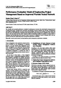
5.0 Example To illustrate the use of SPE•ED for modeling and evaluating the performance of object-oriented systems, we present an example based on a simple automated teller machine (ATM). The ATM accepts a bank card and requests a personal identification number (PIN) for user authentication. Customers can perform any of three transactions at the ATM: deposit cash to an account, withdraw cash from an account, or request the available balance in an account. A customer may perform several transactions during a single ATM session. The ATM communicates with a computer at the host bank which verifies the account and processes the transaction. When the customer is finished using the ATM, a receipt is printed for all transactions and the customer’s card is returned. Here, we focus on scenarios that describe the use of the ATM. A full specification would include additional models, such as a class diagram and behavior descriptions for each class. However, our interest here is primarily in the use of scenarios as a bridge between Object-Oriented Development and Software Performance Engineering. Thus, these additional models are omitted. 5.1 Example Scenarios As described in [Williams and Smith, 1995], scenarios represent a common point of departure between object-oriented requirements or design models and SPE models. Scenarios may be represented in a variety of ways [Williams, 1994]. Here, we use Message Sequence Charts (MSCs) to describe scenarios in object-oriented models. The MSC notation is specified in ITU standard Z.120 [ITU, 1996]. Several other notations used to represent scenarios are based on MSCs (examples include: Event Flow Diagrams [Rumbaugh, et al., 1991]; Interaction Diagrams [Jacobson, et al., 1992], [Booch, 1994]; and Message Trace Diagrams [Booch and Rumbaugh, 1995]). However, none of these incorporates all of the features of MSCs needed to establish the correspondence between object-oriented scenarios and SPE scenarios. Figure 1 illustrates a high-level MSC for the ATM example. Each object that participates in the scenario is represented by a vertical line or axis. The axis is labeled with the object name (e.g., anATM). The vertical axis represents relative time which increases from top to bottom; an axis does not include an absolute time scale. Interactions between objects (events or operation invocations) are represented by horizontal arrows. Figure 1 describes a general scenario for user interaction with the ATM. The rectangular areas labeled “loop” and “alt” are known as “inline expressions” and denote repetition and alternation. This Message Sequence Chart indicates that the user may repeatedly select a transaction which may be a deposit, a withdrawal, or a balance inquiry. The rounded rectangles are “MSC references” which refer to other MSCs. The use of MSC references allows horizontal expansion of Message Sequence

msc userInteraction aUser

anATM

hostBank

cardInserted requestPIN pINEntered

loop

requestTransaction response

alt processDeposit processWithdrawal processBalanceInquiry

terminateSession

Figure 1. Message Sequence Chart for User Interaction with the ATM msc processWithdrawal aUser

anATM

hostBank

requestAccount account requestAmount amount requestAuthorization authorization dispense(amount) requestTakeCash cashTaken transactionComplete ack

Figure 2. Message Sequence Chart processWithdrawal

Charts. The MSC that corresponds to ProcessWithdrawal is shown in Figure 2. A Message Sequence Chart may also be decomposed vertically, i.e., a refining MSC may be attached to an instance axis. Figure 3 shows a part of the decomposition of the anATM instance axis. The dashed arrows represent object instance creation or destruction. 5.2 Mapping Scenarios to Performance Models Models for evaluating the performance characteristics of the proposed ATM system are based on performance scenarios for the major uses of the system. These performance scenarios are the same as the functional scenarios illustrated in the message sequence charts (Figures 1 through 3). However, they are represented using Execution Graphs. Note that not all functional scenarios are necessarily significant msc anATM anATM

aCustomerSession

aWithdrawal

cardInserted new requestPin pINEntered requestTransaction requestTransaction response response new requestAccount requestAccount account account requestAmount requestAmount amount amount requestAuthorization requestAuthorization authorization authorization

...

...

...

Figure 3. Partial Decomposition of anATM

Get customer ID from card

Get PIN from customer

n

Process Transaction

=

Get Transaction

Process Request

Process Deposit Process Withdrawal Process BalanceInquiry

Process Transaction

Terminate Session

Figure 4. Execution graph from ATM Scenario from a performance perspective. Thus, an SPE study would only model those scenarios that represent user tasks or events that are significant to the performance of the system. Figure 4 shows an Execution Graph illustrating the general ATM scenario. The case node indicates a choice of transactions while the repetition node indicates that a session may consist of multiple transactions. Subgraphs corresponding to the expanded nodes show additional processing details. The processing steps (basic nodes) correspond to steps in the lowest-level Message Sequence Chart diagram for the scenario. The execution graph in Figure 4 shows an end-to-end session that spans several ATM customer interactions. Thus analysts can evaluate the performance for each individual customer interaction as well as the total time to complete a session. 3

5.3 Performance Evaluation with SPE•ED After identifying the scenarios and their processing steps in the MSC, the analyst uses SPE•ED to create and evaluate the execution graph model. Figure 5 shows the SPE•ED screen. The “world view” of the model appears in the small navigation boxes on the right side of the screen. The correspondence between an expanded node and its subgraph is shown through color. For example, the top level of the model is in the top-left navigation box; its nodes are black. The top-right (turquoise) navigation box contains the loop to get the transaction and process it. Its corresponding expanded node in the top-level model is also turquoise. The ProcessWithdrawal subgraph is in 3

Some performance analysts prefer to evaluate a traditional “transaction” -- the processing that occurs after a user presses the enter key until a response appears on the screen. This eliminates the highly variable, user-dependent time it takes to respond to each prompt. While that approach was appropriate for mainframe transaction based applications, the approach prescribed here is better for client/server and other distributed systems with graphical user interfaces. The screen design and user interaction patterns may introduce end-to-end response time problems even though computer resource utilization is low.

Specify:

OK

Expand

Overhead

Overhead

©1993 Performance EngineeringServices

Save ScenarioOpen scenario

Trans. complete

Wait for cust to take cash

Dispense cash

Request auth. from hostBank

Get amount

Get account

Process Withdrawal

SPE databaseSysmod globals

System modelService level

Values

Results

Software modNames

Display:

Solve

Insert node

Link

Add

OOD Example

Software model

SPE•ED

TM

Figure 5. SPE•ED Screen with processWithdrawal Subgraph

the large area of the screen (and in the second row, left navigation box). Users can directly access any level in the model by clicking on the corresponding navigation box. The next step is to specify software resource requirements for each processing step. The software resources we examine for this example are: • • • •

Screens - the number of screens displayed to the ATM customer (aUser) Home - the number of interactions with the hostBank Log - the number of log entries on anATM machine Delay - the relative delay for the ATM customer (aUser) to respond to a prompt, or the time for other ATM device processing such as the cash dispenser or receipt printer.

Up to five types of software resources may be specified. The set of five may differ for each subgraph if necessary to characterize performance. The SPE•ED user provides values for these requirements for each processing step in the model, as well as the probability of each case alternative and the number of loop repetitions. The specifications may include parameters that can be varied between solutions, and may contain arithmetic expressions. Resource requirements for expanded nodes are in the processing steps in the corresponding subgraph. The software resource requirements for the ProcessWithdrawal subgraph are in Figure 5. Note that the DispenseCash step displays a screen to inform the customer to take the cash, logs the action to the ATM’s disk, and has a delay for the cash dispenser. We arbitrarily assume this delay to be 5 time units. In the software model the delay is relative to the other processing steps; e.g., the delay for the customer to remove the cash is twice as long as DispenseCash. The user may specify the duration of a time unit (in the overhead matrix) to evaluate the effect on overall performance; e.g., a range of .1 sec. to 2 sec. per time unit. In this example a time unit is 1 sec. The ATM scenario focuses on processing that occurs on the ATM. However, the performance of anATM unit is seldom a performance problem. The SPE•ED evaluation will examine the performance at a hostBank that supports many ATM units.

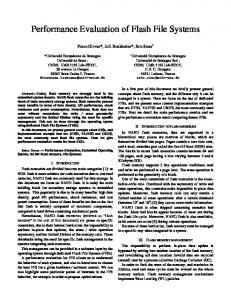
5.4 Processing Overhead SPE•ED supports the SPE process defined in [Smith, 1990]. Analysts specify values for the software resource requirements for processing steps. The computer resource requirements for each software resource request are specified in an overhead matrix stored in the SPE database. This matrix is used for all software models that execute in that hardware/software environment. Figure 6 shows the overhead matrix for this case study. The matrix connects the values specified in the “ATM Spec Template” software specification template with the device usage in the “Host Bank” computer facility. The software resources in the template are in the left column of the matrix; the devices in the facility are in the other columns. The values in the matrix describe

Software spec template: ATM Spec Template

Facility template: Host Bank

Devices Quantity Service units Screen HomeBank Log Delay

Service time

CPU 1 K Instr.

1500

1e-05

ATM Disk 1 200 Screens Phys I/O 1 0.1 0.01 1

1

8

0.02

Figure 6. Overhead Matrix

the device characteristics. The pictures of the devices in the facility are across the top of the matrix, and the device name is in the first row. The second row specifies how many devices of each type are in the facility. For example, if the facility has 20 disk devices, there is one disk device column with 20 in its quantity row. SPE•EDs (deliberately) simple models will assume that disk accesses can be evenly spread across these devices. The third row is a comment that describes the service units for the values specified for the software processing steps. The next five rows are the software resources in the specification template. This example uses only four of them. The last row specifies the service time for the devices in the computer facility. The values in the center section of the matrix define the connection between software resource requests and computer device usage. The screen display occurs on anATM unit; its only affect on the hostBank is a delay. The 1 in the ATM column for the ‘Screen’ row means that each screen specified in the software model causes one visit to the ATM delay server. We arbitrarily assume this delay to be one second (in the service time row). Similarly, each log and delay specification in the software model result in a delay between hostBank processing requests. We assume the log delay is

0.01 seconds. The delays due to processing at the ATM unit could be calculated by defining the overhead matrix for the ATM facility and solving the scenario to calculate the time required. This example assumes that all ATM transactions are for this hostBank; they do not require remote connections. This version of the model assumes 1500 K Instructions execute on the host bank’s CPU (primarily for data base accesses), 8 physical I/Os are required, and a delay of 0.1 seconds for the network transmission to the host bank. These values may be measured, or estimates could be obtained by constructing and evaluating more detailed models of the host processing required. Thus each value specified for a processing step in the software model generates demand for service from one or more devices in a facility. The overhead matrix defines the devices used and the amount of service needed from each device. The demand is the product of the software model value times the value in the overhead matrix cell times the service time for the column.

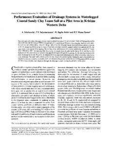
5.5 Model Solutions and Results The analyst first solves a ‘No Contention’ model to confirm that in the best case, a single ATM session will complete in the desired time, without causing performance bottlenecks at the host bank. Up to four sets of results may be displayed concurrently, as shown in Figure 7. The elapsed time result for the ‘No Contention’ model is in the top-left quadrant. The overall time is at the top, and the time for each processing step is next to the step. The color bar legend in the upper right corner of the quadrant shows the values associated with each color; the upper bound is set by defining an overall performance objective. Values higher than the performance objective will be red, lower values are respectively cooler colors. The ‘Resource usage’ values below the color bar legend show the time spent at each computer device. Of the 35.6 total seconds for the endto-end scenario, 35.25 is due to the delays at the ATM unit for customer interactions and processing. Thus, no performance problems are apparent with this result. The SPE tool evaluates the results of device contention delays by automatically creating and solving an analytic queueing network model. The utilization result for the ‘Contention solution’ of the ATM sessions with an arrival rate of 5 withdrawal transactions per second is in the top-right quadrant of Figure 7. The total utilization of each server is shown under the color bar, and the utilization of each device by each processing step is next to the step. The total CPU utilization is 15%, and the disk device is 100%. Even though the customer data base would fit on one disk device, more are needed to relieve the contention delays. In general, options for correcting bottlenecks are to reduce the number of I/Os to the disk, reduce the number of ATM units that share a host bank server, or add disks to the server. The options are evaluated by changing software processing steps, or values in the overhead matrix.

ATM example

ATM example

Time, no contention: 35.6000 Get 1.0000 cust ID

Get PIN1.0100 from

< 2.000 < 3.000 < 4.000 < 5.000 ≥ 5.000 Resource Usage 0.0300 CPU 35.2500 ATM 0.3200 DEV1

Each

Resource utilization: CP Get AT cust ID DE

0.00 0.03 0.00

CP Get PINAT from DE

0.00 0.03 0.00

< 0.250 < 0.500 < 0.750 < 1.000 ≥ 1.000 Model totals 0.15 CPU 0.88 ATM 1.00 DEV1

Each

Get 19.5800 type

CP Get AT type DE

0.15 0.48 1.60

Termina 14.0100 te

CP TerminaAT DE te

0.00 0.35 0.00

Lock ReplaceDelete Print

Lock ReplaceDelete Print

ATM example

ATM example < 0.250 < 0.500 < 0.750 < 1.000 ≥ 1.000

Resource utilization: CP Get AT cust ID DE

0.00 0.03 0.00

CP Get PINAT from DE

0.00 0.03 0.00

Get 1.0000 cust ID

Model totals 0.15 CPU 0.88 ATM 0.53 DEV1

Each

< 1.250 < 2.500 < 3.750 < 5.000 ≥ 5.000

Residence Time: 35.9710

Resource Usage Get PIN1.0100 from

0.0353 CPU 35.2500 ATM 0.6857 DEV1

Each

CP Get AT type DE

0.15 0.48 0.53

Get 19.9510 type

CP TerminaAT DE te

0.00 0.35 0.00

Termina 14.0100 te

Lock ReplaceDelete Print

Lock ReplaceDelete Print

Figure 7. SPE Model Results

The results in the lower quadrants of Figure 7 show the utilization and response time results for 3 disk devices. The quadrants let the analyst easily compare performance metrics for alternatives.

5.6 System Execution Model The ‘System model solution’ creates a queueing network model with all the scenarios defined in a project executing on all their respective facilities. The system execution model picture is in Figure 8. This example models one workload scenario: a session with one withdrawal transaction. The host bank may have other workloads such as teller transactions, bank analyst inquiries, etc. Each performance scenario in the SPE database appears across the top of the system execution model screen. The specification template beside the scenario name displays the current workload intensity and priority. Below the scenario is a template that represents the devices in the facility assigned to the scenario. The facilities in the SPE database appear across the bottom of the system execution model screen. This example models only one facility for the host bank. It could also model the ATM unit, other home banks, etc. The model is solved by calculating the model parameters from the software model for each scenario and then constructing and evaluating a CSIM simulation model [Schwetman, 1994]. CSIM is a simulation product that is widely used to evaluate distributed and parallel processing systems. By automatically creating the models, SPE•ED eliminates the need to code CSIM models in the C programming language. The model results show: • • •

the response time for the scenario and its corresponding color (inside the scenario name rectangle), the amount of the total response time spent at each computer device (the values and colors in the template below the scenario name) the average utilization of each device in each facility and its corresponding color.

One of the model scenarios may be a focus scenario, usually a scenario that is vital to the system development project. Users may view various system model results for processing steps in the focus scenario in 2 quadrants below the system model. One of the difficult problems in simulation is determining the length of the simulation run. SPE•ED solves this problem with the performance results meter shown in Figure 9. It is based on work by [Raatikainen, 1993] adapted for SPE evaluations. The approach is adapted because results depend on the precision of the model parameters, and in early life cycle stages only rough estimates are available. Users may monitor simulation progress and stop the simulation to view results at any point. They may also set a confidence value or simulated run time to automatically terminate the simulation. The meter shows the progress of the current confidence; it is calculated with a batch-mean method. SPE•ED uses a default value of 70% probability that the reported response is within 30% of the actual mean. This bound is much looser than

OOD Example

Utilization: < 0.250 < 0.500 < 0.750 < 1.000 ≥ 1.000

ATM exampl e 0.122 0.754 0.431 0.000

Utilization:

0.43

0.12

Host Bank Lock

Replace

ATM example

Delete

Print

ATM example < 1.250 < 2.500 < 3.750 < 5.000 ≥ 5.000

Residence Time: 21.5388 Get 0.6046 cust ID

Resource Usage Get PIN0.6107 from

0.0198 CPU 21.3131 ATM 0.2060 DEV1

Each

< 0.250 < 0.500 < 0.750 < 1.000 ≥ 1.000

Resource utilization: CP Get AT cust ID DE

0.00 0.02 0.00

CP Get PINAT from DE

0.00 0.02 0.00

Model totals 0.12 CPU 0.75 ATM 0.43 DEV1

Each

Get 11.8527 type

Termina 8.4708 te

Lock ReplaceDelete Print

CP Get AT type DE

0.12 0.41 0.43

CP TerminaAT DE te

0.00 0.30 0.00

Lock ReplaceDelete Print

Figure 8. System Execution Model Results

Simulation progress Sim. time: 443.77 Completions 98

Confidence ±c * Response c:

Stop criteria: Confidence

——

Equal

——

0.1

——

0.2

——

0.3

——

0.4

——

0.5

0.300000 Stop time 5000 Change

Stop

Cancel

Figure 9. Interactive Simulation Control

typically used for computer system models. We selected this value empirically by studying the length of time required for various models, versus the analytic performance metrics, versus the precision of the specifications that determine the model parameters. Users may increase the confidence value, but not the probability. It would be easy to add other controls, but experience with our users shows that this approach is sufficient for their evaluations and requires little expert knowledge of simulation controls.

6.0 Summary and Conclusions This paper describes the SPE performance modeling tool, SPE•ED, and its use for performance engineering of object-oriented software. It describes how to use scenarios to determine the processing steps to be modeled, and illustrates the process with a simple ATM example defined with Message Sequence Charts. It then illustrates the SPE evaluation steps supported by SPE•ED. Object-oriented methods will likely be the preferred design approach of the future. SPE techniques are vital to ensure that these systems meet performance requirements. SPE for OOD is especially difficult since functions may require collaboration among many different objects from many classes. These interactions may be obscured by polymorphism and inheritance, making them difficult to trace. Distributing objects over a network compounds the problem. Our approach of connecting performance models and designs with message sequence charts makes SPE performance modeling

of object-oriented software practical. The SPE•ED tool makes it easier for software designers to conduct their own performance studies. Features that de-skill the performance modeling process and make this viable are: • • • •

quick and easy creation of performance scenarios automatic generation of system execution models visual perception of results that call attention to potential performance problems simulation length control that can be adapted to the precision of the model input data.

Other features support SPE activities other than modeling such as SPE database archives, and presentation and reporting of results. Once performance engineers complete the initial SPE analysis with the simple models and ensure that the design approach is viable, they may export the models for use by “industrial strength” performance modeling tools [Smith and Williams, 1995]. As noted in section 5, Message Sequence Charts do not explicitly capture time. However, the close structural correspondence between scenarios expressed in Message Sequence Charts and those using Execution Graphs suggests the possibility of a straightforward translation from analysis/design models to performance scenarios. Standard SPE techniques, such as performance walkthroughs, best-andworst-case analysis, and others, can then be used to obtain resource requirements or time estimates for processing steps. Providing specifications for the overhead matrix still requires expert knowledge of the hardware/software processing environments and performance measurement techniques. Some performance modeling tools provide libraries with default values for the path lengths. If the benchmark studies that led to the library values closely match the new software being modeled, the default values are adequate. Someone must validate the default values with measurements to ensure that they apply to the new software. Thus the expert knowledge is necessary for both tool approaches. It would be relatively easy to build a feature to automatically populate SPE•EDs overhead matrix from customized measurement tool output, but it is not currently a high priority feature. This paper demonstrates the feasibility of applying SPE to object-oriented systems. Future research is aimed at providing a smooth transition between CASE tools for OOD and SPE evaluation tools.

7.0 References [Baldassari, et al., 1989] M. Baldassari, B. Bruno, V. Russi, and R. Zompi, “PROTOB: A Hierarchical Object-Oriented CASE Tool for Distributed Systems,” Proceedings European Software Engineering Conference - 1989, Coventry, England, 1989.

[Baldassari and Bruno, 1988] M. Baldassari and G. Bruno, “An Environment for ObjectOriented Conceptual Programming Based on PROT Nets,” in Advances in Petri Nets, Lectures in Computer Science No. 340, Berlin, Springer-Verlag, 1988, pp. 1-19. [Beilner, et al., 1988] H. Beilner, J. Mäter, and N. Weissenburg, “Towards a Performance Modeling Environment: News on HIT,” Proceedings 4th International Conference on Modeling Techniques and Tools for Computer Performance Evaluation, Plenum Publishing, 1988. [Beilner, et al., 1995] H. Beilner, J. Mäter, and C. Wysocki, “The Hierarchical Evaluation Tool HIT,” in Performance Tools & Model Interchange Formats, vol. 581/1995, F. Bause and H. Beilner, ed., D-44221 Dortmund, Germany, Universität Dortmund, Fachbereich Informatik, 1995, pp. 6-9. [Booch, 1994] G. Booch, Object-Oriented Analysis and Design with Applications, Redwood City, CA, Benjamin/Cummings, 1994. [Booch and Rumbaugh, 1995] G. Booch and J. Rumbaugh, "Unified Method for ObjectOriented Development," Rational Software Corporation, Santa Clara, CA, 1995. [Buhr and Casselman, 1996] R. J. A. Buhr and R. S. Casselman, Use Case Maps for ObjectOriented Systems, Upper Saddle River, NJ, Prentice Hall, 1996. [Buhr and Casselman, 1994] R. J. A. Buhr and R. S. Casselman, "Timethread-Role Maps for Object-Oriented Design of Real-Time and Distributed Systems," Proceedings of OOPSLA '94: Object-Oriented Programming Systems, Languages and Applications, Portland, OR, October, 1994, pp. 301-316. [Buhr and Casselman, 1992] R. J. A. Buhr and R. S. Casselman, "Architectures with Pictures," Proceedings of OOPSLA '92: Object-Oriented Programming Systems, Languages and Applications, Vancouver, BC, October, 1992, pp. 466-483. [Coleman, et al., 1994] D. Coleman, P. Arnold, S. Bodoff, C. Dollin, H. Gilchrist, F. Hayes, and P. Jeremaes, Object-Oriented Development: The Fusion Method, Englewood Cliffs, NJ, Prentice Hall, 1994. [Goettge, 1990] R. T. Goettge, “An Expert System for Performance Engineering of TimeCritical Software,” Proceedings Computer Measurement Group Conference, Orlando FL, 1990, pp. 313-320. [Grummitt, 1991] A. Grummitt, “A Performance Engineer’s View of Systems Development and Trials,” Proceedings Computer Measurement Group Conference, Nashville, TN, 1991, pp. 455-463. [Hrischuk, et al., 1995] C. Hrischuk, J. Rolia, and C. M. Woodside, "Automatic Generation of a Software Performance Model Using an Object-Oriented Prototype," Proceedings of the Third International Workshop on Modeling, Analysis, and Simulation of Computer and Telecommunication Systems, Durham, NC, January, 1995, pp. 399-409. [ITU, 1996] ITU, "Criteria for the Use and Applicability of Formal Description Techniques, Message Sequence Chart (MSC)," International Telecommunication Union, 1996. [Jacobson, et al., 1992] I. Jacobson, M. Christerson, P. Jonsson, and G. Overgaard, ObjectOriented Software Engineering, Reading, MA, Addison-Wesley, 1992. [Raatikainen, 1993] K. E. E. Raatikainen, “Accuracy of Estimates for Dynamic Properties of

Queueing Systems in Interactive Simulation,” University of Helsinki, Dept. of Computer Science Teollisuuskatu 23, SF-00510 Helsinki, Finland, 1993. [Rolia, 1992] J. A. Rolia, “Predicting the Performance of Software Systems,” University of Toronto, 1992. [Rumbaugh, et al., 1991] J. Rumbaugh, M. Blaha, W. Premerlani, F. Eddy, and W. Lorensen, Object-Oriented Modeling and Design, Englewood Cliffs, NJ, Prentice Hall, 1991. [Schwetman, 1994] H. Schwetman, "CSIM17: A Simulation Model-Building Toolkit," Proceedings Winter Simulation Conference, Orlando, 1994. [Smith, 1990] C. U. Smith, Performance Engineering of Software Systems, Reading, MA, Addison-Wesley, 1990. [Smith and Williams, 1993] C. U. Smith and L. G. Williams, "Software Performance Engineering: A Case Study Including Performance Comparison with Design Alternatives," IEEE Transactions on Software Engineering, vol. 19, no. 7, pp. 720-741, 1993. [Smith and Williams, 1995] C. U. Smith and L. G. Williams, “A Performance Model Interchange Format,” in Performance Tools and Model Interchange Formats, vol. 581/1995, F. Bause and H. Beilner, ed., D-44221 Dortmund, Germany, Universität Dortmund, Informatik IV, 1995, pp. 67-85. [Turner, et al., 1992] M. Turner, D. Neuse, and R. Goldgar, “Simulating Optimizes Move to Client/Server Applications,” Proceedings Computer Measurement Group Conference, Reno, NV, 1992, pp. 805-814. [Williams, 1994] L. G. Williams, "Definition of Information Requirements for Software Performance Engineering," Technical Report No. SERM-021-94, Software Engineering Research, Boulder, CO, October, 1994. [Williams and Smith, 1995] L. G. Williams and C. U. Smith, "Information Requirements for Software Performance Engineering," in Quantitative Evaluation of Computing and Communication Systems, Lecture Notes in Computer Science, vol. 977, H. Beilner and F. Bause, ed., Heidelberg, Germany, Springer-Verlag, 1995, pp. 86-101.