Oct 20, 2014 - cluster.shtml. 2http://www.cscs.ch/computers/piz daint/index.html ..... V. Eijkhout, R. Pozo, C. Romine, and H. V. der Vorst, Templates for the Solution of Linear .... mittee on Computer Architecture (TCCA) Newsletter, p. 19, 1995.
Performance Engineering of the Kernel Polynomial Method on Large-Scale CPU-GPU Systems
arXiv:1410.5242v1 [cs.CE] 20 Oct 2014
Moritz Kreutzer, Georg Hager, Gerhard Wellein Erlangen Regional Computing Center Friedrich-Alexander University of Erlangen-Nuremberg Erlangen, Germany {moritz.kreutzer, georg.hager, gerhard.wellein}@fau.de
Abstract—The Kernel Polynomial Method (KPM) is a wellestablished scheme in quantum physics and quantum chemistry to determine the eigenvalue density and spectral properties of large sparse matrices. In this work we demonstrate the high optimization potential and feasibility of peta-scale heterogeneous CPU-GPU implementations of the KPM. At the node level we show that it is possible to decouple the sparse matrix problem posed by KPM from main memory bandwidth both on CPU and GPU. To alleviate the effects of scattered data access we combine loosely coupled outer iterations with tightly coupled block sparse matrix multiple vector operations, which enables pure data streaming. All optimizations are guided by a performance analysis and modelling process that indicates how the computational bottlenecks change with each optimization step. Finally we use the optimized node-level KPM with a hybrid-parallel framework to perform large scale heterogeneous electronic structure calculations for novel topological materials on a petascale-class Cray XC30 system. Keywords-Parallel programming, Quantum mechanics, Performance analysis, Sparse matrices
I. I NTRODUCTION It is widely accepted that future supercomputer architectures will change considerably compared to the machines used at present for large scale simulations. Extreme parallelism, use of heterogeneous compute devices and a steady decrease in the architectural balance in terms of main memory bandwidth vs. peak performance are important factors to consider when developing and implementing sustainable code structures. Accelerator based systems today already account for a performance share of 35% of the total TOP500 [1] and they may provide first blueprints of future architectural developments. The heterogeneous hardware structure typically calls for a complete new software development – in particular if the simultaneous use of all compute devices is addressed to maximize performance and energy. A prominent example demonstrating the need for new software implementations and structures is the MAGMA project [2]. In dense linear algebra the computational balance of basic operations, e.g. dense matrix-matrix-multiply (GEMM), can often be adapted by blocking techniques to machine balance. Thus, this community is expected to achieve high performance ratios also on future supercomputers. In contrast, sparse linear algebra is known for low sustained per-
Andreas Pieper, Andreas Alvermann, Holger Fehske Institute of Physics Ernst Moritz Arndt University of Greifswald Greifswald, Germany {pieper, alvermann, fehske}@physik.uni-greifswald.de
formance on state of the art homogeneous systems. The sparse matrix vector multiplication (SpMV) is often the performance critical step. Most of the broad research on optimal SpMV data structures has been devoted to drive the balance of general SpMV operations down to its minimum value of 6 Bytes/Flop (double precision) or 2.5 Bytes/Flop (double complex) on all architectures, being at least an order of magnitude away from current hardware balance numbers. Just recently the long known idea of applying the sparse matrix to multiple vectors at the same time (SpMMV), e.g. see [3], to reduce computational balance has gained new interest. A representative of the numerical sparse linear algebra schemes used in natural science applications that can benefit from SpMMV is the Kernel Polynomial Method (KPM). KPM was originally devised for the computation of eigenvalue densities and spectral functions [4], and soon found applications throughout physics and chemistry (see [5] for a review). KPM can be broadly classified as a polynomial-based expansion scheme, with the corresponding simple iterative structure of the basic algorithm that addresses the large sparse matrix from the application exclusively through SpMVs. Recent applications of KPM include, e.g., eigenvalue counting for predetermination of sub-space sizes in projection-based eigensolvers [6] or for large scale data analysis [7]. In this paper we present for the first time a structured performance engineering process for the KPM which substantially brings down the computational balance of the method leading to high sustained performance on CPU and GPU. We apply a data parallel approach for combined CPU-GPU parallelization and present the first large scale heterogeneous CPU-GPU computations for KPM. The main contributions of our work which are of broad interest beyond the original KPM community are as follows: We achieve a systematic reduction of minimal code balance for a widely used sparse linear algebra scheme by implementing a tailored algorithm-specific (“augmented”) SpMV routine instead of relying on a series of sparse linear algebra routines taken from an optimized general library like BLAS and by reformulating the algorithm to use SpMMV to combine loosely coupled outer iterations. Our systematic performance analysis for the SpMMV operation on both CPU and GPU indicates that SpMMV decouples from main memory bandwidth for
sufficiently large vector blocks. It shows that data cache access then becomes a major bottleneck on both architectures. Finally, we demonstrate the feasibility of large scale CPU-GPU KPM computations for a technologically highly relevant application scenario, namely topological materials. In our experiments, the augmented SpMMV KPM version achieves more than 100 TFlop/s on 1024 nodes of a CRAY XC30 system, being equivalent to almost 10 % of aggregated CPU-GPU peak performance. A. Related Work SpMV has been – and still is – a highly relevant subject of research due to the wide appearance of this operation in applications of computational science and engineering. It has turned out that the sparse matrix storage format is a critical factor for SpMV performance. Fundamental research on sparse matrix formats for the architectures considered in this work has been conducted by Barrett et al. [8] for cache-based CPUs and Bell et al. [9] for GPUs. The assumption that efficient sparse matrix storage formats are dependent on and exclusive to a specific architecture has been refuted by Kreutzer et al. [10] by showing that a unified format, namely SELL-C-σ, can yield high performance on both architectures under consideration in this work. Vuduc [11] provides a comprehensive overview of optimization techniques for SpMV. Early research on performance bounds for SpMV and SpMMV has been done by Gropp et al. [3] who established a performance limit taking into account both memory- and instruction-boundedness. A similar approach has been pursued by Liu et al. [12], who established a finer yet similar performance model for SpMMV. Further refinements to this model have been accomplished by Aktulga et al. [13], who did not only consider memory- and instruction-boundedness but also bandwidth bounds of two different cache levels. On the GPU side, literature about SpMMV is scarce. The authors of [9] mention the potential performance benefits of SpMMV over SpMV in the outlook of their work. Anzt et al. [14] have recently presented a GPU implementation of SpMMV together with performance and energy results. The fact that SpMMV is implemented in the library cuSPARSE [15] which is shipped together with the CUDA toolkit proves the relevance of this operation. Optimal usage patterns for heterogeneous supercomputers have become an increasingly important topic with the emergence of those architectures. An important attempt towards high performance heterogeneous execution is MAGMA [2]. However, the hybrid functions delivered by this toolkit are restricted to dense linear algebra. Furthermore, task based work distribution is used in MAGMA, in contrast to the symmetric data-parallel approach used in this work. Matam et al. [16] have implemented a hybrid CPU/GPU solver for sparse matrix-sparse matrix multiplication. However, they do not scale their approach to several heterogeneous nodes. Zhang et al. [17] have presented a KPM implementation for a single NVIDIA GPU, which is not following the conventional data parallel approach. Memory footprint and corre-
sponding main memory access volume of their implementation scale linearly with the number of active CUDA blocks, which limits applicability and performance severely. B. Application Scenario: Topological Materials To support our performance analysis with benchmark data from a real application we will apply our improved KPM implementation to a problem of current interest, the determination of electronic structure properties of a three-dimensional (3D) topological insulator. Topological insulators have found increasing interest in the physics community during the last decade, forming one of the novel material classes similar to graphene with promising applications in fundamental research and technology [18]. The hallmark of these materials is the existence of topologically conserved quantum numbers, which are related to the familiar winding number from two-dimensional geometry, or to the Chern number of the integer quantum Hall effect. The existence of such strongly conserved quantities makes topological materials first-class candidates for quantum computing and quantum information applications. The theoretical modelling of a typical topological insulator is specified by the Hamilton operator � X � † Γ1 − iΓj+1 Ψn + H.c. Ψn+ˆej H = −t 2 n,j=1,2,3 (1) X � + Ψ†n Vn Γ0 + 2Γ1 Ψn , n
which describes the quantum-mechanical behavior of an electric charge in the material, subject to an external electric potential Vn that is used to create a superlattice structure of quantum dots. The vector space underlying this operator can be understood as the product of a local orbital and spin degree of freedom, which is associated with the 4 × 4 Dirac matrices Γa , and the positional degree of freedom n on the 3D crystalline structure composing the topological insulator. We cite the Hamilton operator for the sake of completeness although its precise form is not relevant for the following investigation. For further details see, e.g., Refs. [19], [20]. From the expression (1) one obtains the sparse matrix representation of the Hamilton operator by choosing appropriate boundary conditions and spelling out the entries of the matrices Γa . Here, we treat finite samples of dimension Nx × Ny × Nz , such that the matrix H in the KPM algorithm has dimension N = 4Nx × Ny × Nz . The number of non-zero entries Nnz ≈ 13N . The matrix has complex entries, but it is hermitian by construction. Characteristic for these applications is the presence of several sub-diagonals in the matrix. Periodic boundary conditions in the x, y direction lead to outlying diagonals in the matrix corners. In the present example, the matrix is a stencil but not a band matrix. Because of the quantum dot superlattice structure translational symmetry is not available to reduce the problem size. This make the current problem relevant for large-scale computations.
4
5 4
DOS / 0.0001
DOS / 0.1
3 2 1
3 2 1
0 -4
-2
0
2
0 -0.15
4
-0.1
-0.05
E
0
0.05
0.1
0.15
E
Fig. 1: DOS for a 1600 × 1600 × 40 topological insulator (N ≈ 4 × 10⁸ ) computed with the KPM-DOS algorithm. 0.1
0.1 D=100
50
0.05
0
0 0
50
100
150
x
1
0
0.1
-0.05 -0.1 -0.04
A(k,E)
100
10
0.05 E
y
0.15 VDot=0.153
LDOS (z=0, E=0)
0.2 R=25
150
0.01 -0.02
0 kx / π
0.02
0.04
Fig. 2: Left panel: Local DOS for a quantum dot superlattice imposed on top of a topological insulator. Right panel: Corresponding momentum-resolved spectral function A(k, E). See, e.g., Refs. [19], [20] for details on the physics.
One basic quantity of interest for physics applications is the eigenvalue density, or density of states (DOS), ρ(E) =
N X
δ(E − En ) = tr[δ(E1 − H)] ,
(2)
n=1
where the sum of the trace tr[. . . ] runs over all eigenvalues En of H. The DOS gives the number of eigenvalues per interval, and can also be used, e.g., to predict the required size of subspaces for eigenvalue projection techniques [6], [21]. A direct method for computation of ρ(E) that uses the first expression in Eq. (2) would have to determine all eigenvalues of H, which is not feasible for large matrices. Instead, we rely on the KPM-DOS algorithm introduced in the next section. In figs. 1, 2 a few data for the DOS obtained with KPM-DOS are shown for the present application. II. P ROBLEM D ESCRIPTION The KPM is a polynomial expansion technique for the computation of spectral quantities of large sparse matrices, see our review [5] for a detailed exposition. In the context of Eq. (2) the KPM does not work directly with the first expression, but with a systematic expansion of the δ-function in the second expression. KPM is based on the orthogonality properties and two-term recurrence for Chebyshev polynomials Tm (x) of the first kind. Specifically, in KPM one successively computes the ˜ 0 i from a starting vector |ν0 i, for vectors |νm i = Tm (H)|ν 1 ≤ m ≤ M/2 with prescribed M , through the recurrence ˜ 0i , |ν1 i = H|ν
˜ m i − |νm−1 i . |νm+1 i = 2H|ν
(3)
˜ only in (sparse) matrixThe recurrence involves the matrix H vector multiplications. Because the Chebyshev polynomials are defined as orthogonal polynomials only on the interval ˜ = a(H−b1) [−1, 1] one must re-scale the original matrix as H
for r = 0 to R − 1 do |vi ← |rand()i Initialization steps and computation of η0 , η1 for m = 1 to M/2 do swap(|wi, |vi) |ui ← H|vi ⊲ spmv() |ui ← |ui − b|vi ⊲ axpy() |wi ← −|wi ⊲ scal() |wi ← |wi + 2a|ui ⊲ axpy() η2m ← hv|vi ⊲ nrm2() η2m+1 ← hw|vi ⊲ dot() end for end for Fig. 3: Naive version of the KPM-DOS algorithm with corresponding BLAS level 1 function calls. Note that the “swap”operation is not performed explicitly, but merely indicates the logical change of the role of the v, w vector in the odd/even iteration steps.
˜ is contained in with a, b ∈ R such that the spectrum of H [−1, 1]. Suitable values of a, b can be determined initially with Gershgorin’s circle theorem or a few Lanczos sweeps. From the vectors |νm i two scalar products η2m = hνm |νm i, η2m+1 = hνm+1 |νm i are computed in each iteration step. Spectral quantities are reconstructed from these scalar products in a second computationally inexpensive step, which is independent of the KPM iteration and needs not be discussed in the context of performance engineering. For the computation of a spectrally averaged quantity, e.g., the DOS from Eq. (2), the trace can be approximated by a sum over several independent PR (r) (r) random initial vectors as in tr[A] ≈ (1/R) r=1 hν0 |A|ν0 i (see [5] for further details). A direct implementation of the above scheme results in the “naive” version of the KPM-DOS algorithm in Fig. 3. One feature of KPM is the very simple implementation of the basic scheme, which leaves substantial headroom for performance optimizations. The above algorithm involves one SpMV and a few BLAS level 1 operations per step. If only two vectors are stored in the implementation the scalar products have to be computed before the next iteration step. That and the multiple individual BLAS level 1 operations on the vectors |vi, |wi call for optimization of the local data access patterns. A careful implementation reduces the amount of global reductions over the dot products to a single one at the end of the inner loop. Furthermore, in its present form, the stochastic trace is performed with an outer loop over R random vectors. Although the inner KPM iterations for different initial vectors are independent of each other, performance gains compared to the embarrassingly parallel version with R independent runs can be achieved by incorporating the “trace” functionality into the parallelized algorithm. see Section VI-C for detailed performance results.
Funct.
# Calls
Min. Bytes/Call
Flops/Call
spmv()
RM/2
Nnz (Fa + Fm )
axpy() scal() nrm2() dot()
RM RM/2 RM/2 RM/2
Nnz (Sd + Si )+ 2N Sd 3N Sd 2N Sd N Sd 2N Sd RM/2[Nnz (Sd + Si ) + 13N Sd ]
KPM
1
N (Fa + Fm ) N Fm N (⌈Fa /2⌉ + ⌈Fm /2⌉) N (Fa + Fm ) RM/2[Nnz (Fa + Fm )+ N (⌈7Fa /2⌉ + ⌈9Fm /2⌉)]
TABLE I: Minimum number of transferred bytes and executed flops for each function involved in Fig. 3. for r = 0 to R − 1 do |vi ← |rand()i Initialization steps and computation of η0 , η1 for m = 1 to M/2 do swap(|wi, |vi) |wi = 2a(H − b1)|vi − |wi & η2m = hv|vi & η2m+1 = hw|vi ⊲ aug_spmv() end for end for Fig. 4: Optimization stage 1: Improved version of the KPMDOS algorithm using the augmented SpMV kernel, which covers all operations chained by ’&’.
III. A LGORITHM A NALYSIS
AND
O PTIMIZATION
To get a first overview of the algorithm’s properties it is necessary to study its requirements in terms of data transfers and computational work, both of which depend on the data types involved. Sd and Si denote the size of a single matrix/vector data element and matrix index element, respectively. Fa (Fm ) indicates the number of floating point operations (flops) per addition (multiplication). Table I shows the minimum number of flops to execute and memory bytes to transfer for each of the operations involved in Fig. 3 and for the entire algorithm. Generally speaking, algorithmic optimization involves a reduction of resource requirements, i.e., lowering either the data traffic or the number of flops. While we assume the latter to be fixed for this algorithm, it is possible to improve on the former. From Fig. 3 it becomes clear that the vectors u, v, and w are read and written several times. An obvious optimization is to merge all involved operations into a single one. This is a simple and widely applied code optimization technique, also known as loop fusion. In our case, we augment the SpMV kernel with the required operations for shifting and scaling. Furthermore, the needed dot products are being calculated on-the-fly in the same kernel. Note that optimizations of this kind usually require manual implementation due to the lack of libraries providing exactly the kernel as needed. The new kernel will be called aug_spmv() and the resulting algorithm is shown in Fig. 4. The data traffic due to the vectors has been reduced in comparison with the naive implementation in Fig. 3 by saving 10 vector transfers in each inner iteration. A further improvement
|V i := |vi0..R−1 ⊲ Assemble vector blocks |W i := |wi0..R−1 |V i ← |rand()i Initialization steps and computation of µ0 , µ1 for m = 1 to M/2 do swap(|W i, |V i) |W i = 2a(H − b1)|V i − |W i & η2m [:] = hV |V i & η2m+1 [:] = hW |V i ⊲ aug_spmmv() end for Fig. 5: Optimization stage 2: Blocked and improved version of the KPM-DOS algorithm using the augmented SpMMV kernel. Now, each η is a vector of R column-wise dot products of two block vectors.
can be accomplished by exploiting that the same matrix H −b1 gets applied to R different vectors. By interpreting the vectors as a single block vector of width R, one can get rid of the outer loop and apply the matrix to the whole block at once. Thus, the resulting operation is an augmented SpMMV, to be referred as aug_spmmv(). The resulting algorithm is shown in Fig. 5. Now the matrix only has to be read M/2 times and the data traffic is reduced further. We summarize the data transfer savings for each optimization stage by showing the evolution of the entire solver’s minimum data traffic VKPM : VKPM = RM/2[Nnz(Sd + Si ) + 13Sd N ] ⇓ Using aug_spmv() = RM/2[Nnz(Sd + Si ) + 3Sd N ] ⇓ Using aug_spmmv() = M/2[Nnz (Sd + Si ) + 3RSd N ].
(4)
A. General Performance Considerations Using VKPM from Eq. (4) and the number of flops as presented in Table I the minimum code balance of the solver is: Nnz (Sd + Si ) + 3RSd N R[Nnz (Fa + Fm ) + N (⌈7Fa /2⌉ + ⌈9Fm /2⌉)] Nnzr /R(Sd + Si ) + 3Sd bytes = . Nnzr(Fa + Fm ) + (⌈7Fa /2⌉ + ⌈9Fm /2⌉) flop
Bmin =
Nnzr = Nnz /N denotes the average number of entries per row which is approximately 13 in our test case. As we are using complex double precision floating point numbers for storing the vector and matrix data, one data element requires 16 bytes of storage (Sd = 16). For storing indices, 4 byte integers are used inside the kernels (Si = 4). Note that the code as a whole uses mixed integer sizes, as for global quantities in large-scale runs, 8 byte indices are necessary. Furthermore, for complex arithmetic it holds that Fa = 2 and Fm = 6. Using the actual
values for the test problem, we arrive at 13/R(16 + 4) + 3 · 16 bytes 13(2 + 6) + (⌈7 · 2/2⌉ + ⌈9 · 6/2⌉) flop 260/R + 48 bytes = (5) 138 flop bytes (6) Bmin (1) ≈ 2.23 flop bytes (7) lim Bmin ≈ 0.35 R→∞ flop Bmin (R) =
Usually the actual code balance is larger than Bmin . This is mostly due to the fact that part of the SpM(M)V input vector is read from main memory more than once. This can be caused by an unfavorable matrix sparsity pattern or an undersized last level cache (LLC). The performance impact can be quantified by a factor Ω = Vmeas /VKPM with Vmeas being the actually transferred bytes as measured with, e.g., LIKWID [22] on CPUs, and NVIDIA’s nvprof [23] profiling tool on NVIDIA GPUs. Thus, the actual code balance results in B = ΩBmin .
(8)
Following the ideas of Gropp et al. [3] and Williams et al. [24], a simple roofline model can be applied for performance modelling and prediction. The roofline model states that an upper bound for the achievable performance of a loop with code balance B can be predicted as the minimum of the theoretical peak performance P peak and the performance limit due to the memory bandwidth b: � � b P ∗ = min P peak , . (9) B The large code balance for R = 1 (Eq. (6)) indicates that the kernel will be memory-bound in this case on modern standard hardware, i.e., the maximum memory-bound performance according to Eq. (9) is b . (10) B An important observation from Eqs. (6) and (7) is that the code balance decreases when going to larger values of R, i.e., when substituting SpMV by SpMMV. In other words: The kernel execution gets more and more independent from the originally relevant bottleneck, i.e. the memory interface. On the other hand, larger vector blocks require more space in the cache which may cause an increase of Ω and an increase of the code balance as a consequence thereof. See [25] for a more detailed analysis of this effect. The application of the roofline model will be discussed in Section V-A. ∗ PMEM =
IV. T ESTBED AND I MPLEMENTATION Table II shows relevant architectural properties like the maximum width of SIMD processing (cf. Section IV-A), the attainable bandwidth b as measured with the STREAM [26] benchmark, the last level cache size LLC, and the theoretical peak double precision floating point performance P peak . Simultaneous multithreading (SMT) has been enabled on the
IVB SNB K20m K20X
Clock (MHz)
SIMD (Bytes)
Cores/ SMX
b (GB/s)
LLC (MiB)
P peak (Gflop/s)
2200 2600 706 732
32 32 512 512
10 8 13 14
50 48 150 170
25 20 1.25 1.5
176 166.4 1174 1311
TABLE II: Architectural properties of all architectures used in this paper: Intel Xeon E5-2660 v2 (“IVB”) with fixed clock frequency, Intel Xeon E5-2670 (“SNB”) with turbo mode enabled, NVIDIA Tesla K20m with ECC disabled, and NVIDIA Tesla K20X with ECC enabled
CPUs, which results in a total thread count of twice the number of cores. Both GPUs implement the “Kepler” architecture where each Streaming Multiprocessor (SMX) features 64 double precision units capable of fused multiply add (FMA). The Intel C Compiler (ICC) version 14 has been used for the CPU code. For the GPU code, the CUDA toolkit 5.5 was employed. Measurements for the node-level performance analysis (Sections V-A and V-B) have been conducted on the Emmy1 cluster at Erlangen Regional Computing Center (RRZE). This cluster contains a number of nodes combining two IVB CPUs with two K20m GPUs. For large-scale production runs we used the heterogeneous petascale cluster Piz Daint2 , a Cray XC30 system located at the Swiss National Computing Centre (CSCS) in Lugano, Switzerland. Each of this system’s 5272 nodes consists of one SNB CPU and one K20X GPU. A. General Notes on the Implementation Although the involved compute platforms are heterogeneous at first sight, they have architectural similarities which allow the application of optimization techniques from which the performance on both architectures can benefit. Within the scope of this work, an important feature in this regard is data parallelism. Modern CPUs feature Single Instruction Multiple Data (SIMD) units which enable parallel processing on the core level. The current Intel CPUs used here implement the AVX instruction set, which contains 256-bit wide vector registers. Hence, four real or two complex numbers can be processed at once in double precision. The equivalent hardware feature on GPUs is called Single Instruction Multiple Threads (SIMT), which can be seen as “SIMD on a thread level.” Here, a group of threads called warp executes the same instruction at a time. On all modern NVIDIA GPUs a warp consists of 32 threads, regardless of the data type. Instruction divergence within a warp causes serialization of the thread execution. In contrast to this, CPU SIMD code has to be entirely uniform in order to work at all. Up to 32 warps are grouped in a thread block, which is the unit of work scheduled on an SMX. 1 https://www.rrze.fau.de/dienste/arbeiten-rechnen/hpc/systeme/emmycluster.shtml 2 http://www.cscs.ch/computers/piz daint/index.html
For an efficient utilization of SIMD/SIMT processing the data access has to be contiguous per instruction. On GPUs, load coalescing (i.e., subsequent threads have to access subsequent memory locations) is crucial for efficient global load instructions. Achieving efficient SIMD/SIMT execution for SpMV is connected to several issues like zero fill-in and the need for gathering the input vector data [10]. For SpMV, vectorized access can only be achieved with respect to the matrix data. However, in the case of SpMMV this issue can be solved since contiguous data access is possible across the vectors. Note that it is necessary to store the vectors in an interleaved (row-major) way for best efficiency. This may not be the case for some applications, i.e., transposing the block vector data layout may be required. An advantage of the vectorization with respect to the vectors is the lack of special requirements on the matrix storage format, because matrix elements can be accessed in a serial manner. Hence, the CRS (similar to SELL-1) data format can be used on both architectures without drawbacks. It is noteworthy that CRS/SELL-1 may yield even better SpMMV performance than a SIMD-aware storage format for SpMV like SELL-32, because matrix elements within a row are stored consecutively. B. CPU Implementation The CPU kernels have been hand-vectorized using AVX compiler intrinsics. A custom code generator was used to create fully unrolled versions of the kernel codes for different combinations of the SELL chunk height and the block vector width. As the AVX instruction set supports 32-byte SIMD units, a minimal vector block width of two is already sufficient for achieving perfectly vectorized access to the (complex) vector data. For memory bound algorithms (like the naive implementation in Fig. 3) and large working sets, efficient vectorization may not be required for optimal performance. However, as discussed in Section III-A, our optimized kernel is no longer strictly bound to memory bandwidth. Hence, efficient vectorization is a crucial ingredient for high performance. To guarantee best results, manual vectorization cannot be avoided, especially in the case of complex arithmetic. C. GPU Implementation The GPU kernels have been implemented using CUDA and hand-tuned for the Kepler architecture. There are well-known approaches for efficient SpMV (see, e.g., [9], [10] and references therein), but the augmented SpMMV kernel requires more effort. In particular for the implementation of on-thefly dot product computations a sensible thread management is crucial. Figure 6 shows how the threads are mapped to the computation in the full aug_spmmv() kernel. For the sake of easier illustration, relevant architectural properties have been set to smaller values. In reality, the warpSize is 32 on Kepler and the maximum (and also the one which is used) blockDim is 1024. The threads in a warp are colored with increasing brightness in the figure. Note that this implementation is optimized towards relatively large vector blocks (R ' 8). In
the following we explain the components of the augmented SpMMV kernel. 1) SpMMV: The first step of the kernel is the SpMMV. In order to have coalesced access to the vector data, the warps must be arranged along block vector rows. Obviously, perfectly coalesced access can only be achieved for block vector widths which are at least as large as the warp size. We have observed, however, that smaller block widths achieve reasonable performance as well. In Fig. 6 the load of the vector data would be divided into two loads using half a warp each. 2) Re-index warps: Operations involving reductions are usually problematic in GPU programming for two reasons: First, reductions across multiple blocks make it necessary to synchronize the threads among the blocks. Second, the reduction inside a block required the use of shared memory for previous NVIDIA architectures, which is no longer true for Kepler, however. This architecture implements shuffle instructions which enable sharing values between threads in a warp without having to use shared memory [27]. For the dot product computation, the values which have to be shared between threads are located in the same vector (column of the block). This access pattern is different from the one as used in step (1), where subsequent threads access different columns of the block. Hence, the thread indexing in the warps has to be adapted. Note that no data actually gets transposed but merely the indexing changes. 3) Dot product: The actual dot product computation consists of two steps. Computing the initial product is trivial, as each thread only computes the product of the two input vectors. For the reduction phase, subsequent invocations of the shuffle instruction as implemented in the Kepler architecture are used. In total, log2 (warpSize) reductions are required for computing the full reduction result, which can then be obtained from the first thread. For the final reduction across vector blocks, CUB [28] has been used (not shown in Fig. 6). V. P ERFORMANCE M ODELS In this section we apply the analysis from Section III-A to both our CPU and GPU implementation using an IVB CPU and a K20m GPU. We use a domain of size 100 × 100 × 40 if not stated otherwhise. This results in a matrix with 1.6 million rows. Thus, neither the matrix nor the vectors fit into any cache on either architecture. A. CPU Performance Model The relevant architectural bottleneck for SpM(M)V changes when increasing the block vector width. This assertion can be confirmed by analyzing the intra-socket scaling performance, which has been done in Fig. 7 for IVB. The assumption that the SpMV kernel is bound to main memory bandwidth is confirmed by the data: The performance saturates at a level (dashed line) which is reasonably close the roofline prediction obtained from Eq. (10). In contrast to this, the SpMMV kernel does not saturate this bottleneck and its performance scales almost linearly within a socket. This indicates that the relevant bottleneck is either the bandwidth of some cache level or the
blockDim=32,
warpSize = 8,
R = 4,
Warp layout:
=
*
t0 t1 t2 t3 t4 t5 t6 t7
(2) Re-index warps
(1) Sparse matrix multiple vector multiplication
*: Only shown for a single vector
* * * * * * * * (3.1) Initial product*
+
+
+
+
+
+ +
(3.2) Intra-warp reduction*
Fig. 6: GPU implementation of SpMMV with on-the-fly dot product. Only a single thread block is shown.
Performance in Gflop/s
80 spmmv_aug(), R=32 spmv_aug()
70 60 50 40 30
Roofline prediction
20 10 0
1
2
3
4
5
6
7
8
9 10
Number of cores
Fig. 7: Socket scaling on IVB. The roofline prediction is a result of using the measured attainable bandwidth b from Table II, the code balance Bmin from Eq. (6), and Ω = 1 (best case) in Eq. (9)
in-core execution. It turns out that taking into account the L3 cache yields sufficient insight for a qualitative analysis of the performance bottlenecks (for recent work on refined roofline models for SpMMV see [13] where both the L2 and L3 cache were considered). The roofline model (Eq. (9)) can be modified by defining a more precise upper performance bound than P peak for non-memory bound codes. Our refined roofline model reads ∗ ∗ P ∗ = min(PMEM , PLLC ).
(11)
∗ PLLC
Here, is a performance limit for the last level cache, which is determined through benchmarking a down-sized problem where the whole working set (matrix and vectors) fits into the L3 cache of IVB while keeping the matrix as similar as possible to the memory-bound test case. A comparison of our custom roofline model with measured performance for the augmented SpM(M)V kernel is shown in Fig. 8. The shift of the relevant bottleneck can be identified: For small R the kernel is memory-bound and the performance can be predicted by the standard roofline model (Eq. (9)) with high accuracy. At larger R, the kernel’s execution decouples from main memory. A high quality performance prediction is more complicated in this region, but our refined model (Eq. (11)) does not deviate by more than 15% from the measurement. A further observation from Fig. 8 is the impact of Ω (see ∗ annotations in the figure) on the code balance and on PMEM . For large R the maximum achievable performance decreases although the minimum code balance (cf. Eq. (5) originally suggests otherwise. B. GPU Performance Model On the GPU, establishing a custom roofline model as in Eq. (11) is substantially more difficult because one can not
use the GPU to full efficiency with a data set which fits in the L2 cache. Hence, the performance model for the GPU will be more of a qualitative nature. The Kepler architecture is equipped with two caches which are relevant for the execution of our kernel. Information on these caches can be found in [27] and [29]: 1) L2 cache: The L2 cache is shared between all SMX units. In the case of SpMV, it serves to alleviate the penalty of unstructured accesses to the input vector. 2) Read-only data cache: On Kepler GPUs there is a 48 KiB read-only data cache (also called texture cache) on each SMX. This cache has relaxed memory coalescing rules, which enables efficient broadcasting of data to all threads of a warp. It can be used in a transparent way if read-only data (such as the matrix and input vector in the aug_spmmv() kernel) is marked with both the const and __restrict__ qualifiers. In the SpMMV kernel, each matrix entry needs to be broadcast to the threads of a warp (see Section IV-C for details), which makes this kernel a very good usage scenario for the read-only data cache. In Section IV-C we have described how the computation of dot products complicates the augmented SpMMV kernel. For our bottleneck analysis we thus consider the plain SpMMV kernel, the augmented SpMMV kernel (but without on-the-fly computation of dot products), and finally the full augmented SpMMV kernel. To quantify the impact of different memory system components we present measured data volumes when executing the simple SpMMV kernel (the qualitative observations are similar for the other kernels) for each of them in Fig. 9. The data traffic coming from the texture cache scales linearly with R because the scalar matrix data is broadcast to the threads in a warp via this cache. The accumulated data volume across all hierarchy levels decreases for increasing R, which is due to the shrinking relative impact of the matrix on the data traffic. A potential further reason for this effect is higher load efficiency in the large R range. Figure 10 shows DRAM, L2 cache, and Texture cache bandwidth measurements for the three kernels mentioned above. At R = 1 the DRAM bandwidth is around 150 GB/s for the first two kernels, which is equal to the maximum attainable bandwidth on this device (see Table II; as expected, the kernel is memory bound. The bandwidths drawn from L2 and Texture cache are not much higher than the DRAM bandwidth in
VI. P ERFORMANCE R ESULTS A. Symmetric Heterogeneous Execution
Performance in Gflop/s
MPI is used as a communication layer for heterogeneous execution and the parallelization across devices is done on a per-process basis. On a single heterogeneous node, simultaneous hybrid execution could also be implemented without MPI. However, using MPI already on the node level enables easy scaling to multiple heterogeneous nodes and portability to other heterogeneous systems. We use one process for each CPU/GPU in a node and OpenMP within CPU processes. A GPU process needs a certain amount of CPU resources for executing the host code and calling GPU kernels, for which one CPU core is usually sufficient. Hence, for the heterogeneous measurements in this paper one core per socket was “sacrificed” to its GPU. Each process runs in its own 100
100
80
80 Ω = 1.16
60
Ω
.1