Performance Evaluation Metrics and Statistics for Positional Tracker ...

Performance Evaluation Metrics and Statistics for Positional Tracker Evaluation Chris J. Needham and Roger D. Boyle School of Computing, The University of Leeds, Leeds, LS2 9JT, UK {chrisn,roger}@comp.leeds.ac.uk http://www.comp.leeds.ac.uk/chrisn

Abstract. This paper discusses methods behind tracker evaluation, the aim being to evaluate how well a tracker is able to determine the position of a target object. Few metrics exist for positional tracker evaluation; here the fundamental issues of trajectory comparison are addressed, and metrics are presented which allow the key features to be described. Often little evaluation on how precisely a target is tracked is presented in the literature, with results detailing for what percentage of the time the target was tracked. This issue is now emerging as a key aspect of tracker performance evaluation. The metrics developed are applied to real trajectories for positional tracker evaluation. Data obtained from a sports player tracker on video of a 5-a-side soccer game, and from a vehicle tracker, is analysed. These give quantitative positional evaluation of the performance of computer vision tracking systems, and provides a framework for comparison of different methods and systems on benchmark data sets.

1

Introduction

There are many ways in which the performance of a computer vision system can be evaluated. Often little evaluation on how precisely a target is tracked is presented in the literature, with the authors tending to say for what percentage of the time the target was tracked. This problem is beginning to be taken more seriously, and an annual workshop on performance evaluation of tracking and surveillance [5] has begun recently (2000). Performance evaluation is a wide topic, and covers many aspects of computer vision. Ellis [1] discusses approaches to performance evaluation, and covers the different areas, which include how algorithms cope in different physical conditions in the scene, i.e. weather, illumination and irrelevant motion, to assessing performance through ground truthing and the need to compare tracked data to marked up data, whether this be targets’ positions, 2D shape models, or classification of some description. In previous work [4] , mean and standard deviations of errors in tracked data from manually marked up data has been presented, with simple plots. Harville [2] presents similar positional analysis when evaluating the results of person tracking using plan-view algorithms on footage from stereo cameras. In certain J.L. Crowley et al. (Eds.): ICVS 2003, LNCS 2626, pp. 278–289, 2003. c Springer-Verlag Berlin Heidelberg 2003


Performance Evaluation Metrics and Statistics

279

situations Dynamic Programming can be applied to align patterns in feature vectors, for example in the speech recognition domain as Dynamic Time Warping (DTW) [6]. In this work trajectory evaluation builds upon comparing equal length trajectories having frame by frame time steps with direct correspondences. When undertaking performance evaluation of a computer vision system, it is important to consider the requirements of the system. Common applications include detection (simply identifying if the target object is present), coarse tracking (for surveillance applications), tracking (where reasonably accurate locations of target objects are identified), and high-precision tracking (for medical applications, reconstructing 3D body movements). This paper focuses on methods behind positional tracker evaluation, the aim being to evaluate how well a tracker is able to determine the position of a target object, for use in tracking and high-precision tracking as described above.

2

Metrics and Statistics for Trajectory Comparison

Few metrics exist for positional tracker evaluation. In this section the fundamental issues of trajectory comparison are addressed, and metrics are presented which allow the key features to be described. In the following section, these metrics are applied to real trajectories for positional tracker evaluation. 2.1

Trajectory Definition

A trajectory is a sequence of positions over time. The general definition of a trajectory T is a sequence of positions (xi , yi ) and corresponding times, ti : T = {(x1 , y1 , t1 ), (x2 , x2 , t2 ), . . . , (xn , yn , tn )}

2

3

4 4

1 2 1

5 5

6 6

7 7

(1)

8 8

3

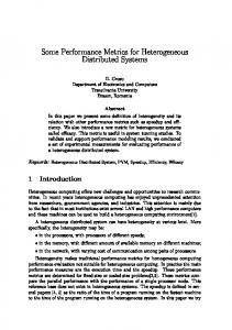
Fig. 1. Example of a pair of trajectories.

In the computer vision domain, when using video footage, time steps are usually equal, and measured in frames. Thus, tn may be dropped, as the subscript on the positions can be taken as time, and Equation 1 becomes: T = {(x1 , y1 ), (x2 , x2 ), . . . , (xn , yn )}

(2)

280

C.J. Needham and R.D. Boyle

i.e. trajectory T is a sequence of (xi , yi ) positions at time step i, as illustrated in Figure 1. Paths are distinguished from trajectories by defining a path as a trajectory not parameterised by time. To evaluate the performance of the tracker, metrics comparing two trajectories need to be devised. We have two trajectories TA and TB which represent the trajectory of a target from the tracker, and the ground truth trajectory which is usually marked up manually from the footage. Metrics comparing the trajectories allow us to identify how similar, or how different they are. 2.2

Comparison of Trajectories

Consider two trajectories composed of 2D positions at a sequence of time steps. Let positions on trajectory TA be (xi , yi ), and on trajectory TB be (pi , qi ), for each time step i. The displacement between positions at time step i is given by di : di = (pi , qi ) − (xi , yi ) = (pi − xi , qi − yi ) And the distances between the positions at time step i are given by di :
di = |di | = (pi − xi )2 + (qi − yi )2

(3)

(4)

Fig. 2. Comparison of displacement between two trajectories.

A metric commonly used for tracker evaluation is the mean of these distances [4,2]. We shall call this metric m1 . n

m1 = µ(di ) =

1 di n i=1

(5)

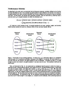
m1 gives the average distance between positions at each time step. Figure 2 shows two trajectories and identifies the distance between corresponding positions. The distribution of these distances is also of significance, as it shows how the distances between trajectories (tracker error) are spread, as illustrated in Figure 3, where a skewed distribution can be seen. Other statistics provide quantitative information about the distribution. Here we identify the mean, median (expected to be lower than the mean, due to the

Performance Evaluation Metrics and Statistics

Relative Frequency

0.004

281

Errors in Hand Tracking

0.003

0.002

0.001

0 0

1000

2000

Error Measured as Euclidean Distance in mm

Fig. 3. Distribution of distances between positions.

contribution to the mean of the furthest outliers), standard deviation, minimum and maximum values as useful statistics for describing the data. Let us define D(TA , TB ) to be the set of distances di between trajectory A and B. The above statistics can be applied to this set: n µ( D(TA , TB ) ) = n1 i=1 di median( D(TA , TB ) ) = d n+1 if n odd, 2 1 n + dn = (d ) if n even +1 2 2 n 2 1 Standard deviation σ( D(TA , TB ) ) = n i=1 (di − µ(di ))2 Minimum min( D(TA , TB ) ) = the smallest di Maximum max( D(TA , TB ) ) = the largest di (6) Mean Median

2.3

Spatially Separated Trajectories

Some pairs of trajectories may be very similar, except for a constant difference in some spatial direction (Figure 4). Defining a metric which takes this into account may reveal a closer relationship between two trajectories.

6

4 2

7

5

3

1 4 2

3

6 5

7

1

Fig. 4. Two spatially separated trajectories.

282

C.J. Needham and R.D. Boyle

Given the two trajectories TA and TB , it is possible to calculate the optimal ˆ (shift) of TA towards TB , for which m1 is minimised. d ˆ is spatial translation d the average displacement between the trajectories, and is calculated as: n

 ˆ = µ(di ) = 1 d di n i=1

(7)

ˆ TB ) to be the set of distances between a translated Now we can define D(TA + d, ˆ and TB . The same statistics can be applied to this set, trajectory TA (by d) ˆ TB ), to describe the distances. µ( D(TA + d, ˆ TB ) ) < µ( D(TA , TB ) ) D(TA + d, in all cases, except when the trajectories are already optimally spatially aligned. ˆ TB ) ) is significantly lower than µ( D(TA , TB ) ), it may When µ( D(TA + d, highlight a tracking error of a consistent spatial difference between the true position of the target, and the tracked position. 2.4

Temporally Separated Trajectories

Some pairs of trajectories may be very similar, except for a constant time difference (Figure 5). Defining a metric which takes this into account may reveal a closer relationship between two trajectories.

7 5 6 3 1

21

4 34 2

5 6

7

Fig. 5. Two temporally separated trajectories.

Given the two trajectories TA and TB , it is possible to calculate the optimal temporal translation j (shift) of TA towards TB , for which m1 is minimised. When the time-shift j is positive TA,i is best paired with TB,i+j , and when j is positive TA,i+j is best paired with TB,i . Time-shift j is calculated as:  j = arg mink

R   1 |(pi+k , qi+k ) − (xi , yi )| n − |k| i=Q

(8)

if k
0 then Q = 0 else Q = −k. R = Q + n − |k|. Now we can define D(TA , TB , j) to be the set of distances between a temporally translated trajectory TA or TB , depending on j’s sign. The same statistics as before can be applied to this set, D(TA , TB , j), to describe the distances.

Performance Evaluation Metrics and Statistics

283

µ( D(TA , TB , j) ) < µ( D(TA , TB ) ) in all cases, except when the trajectories are already optimally temporally aligned. When µ( D(TA , TB , j) ) is significantly lower than µ( D(TA , TB ) ), it may highlight a tracking error of a consistent temporal difference between the true position of the target, and the tracked position. In practice j should be small; it may highlight a lag in the tracked position (Figure 5). 2.5

Spatio-Temporally Separated Trajectories

Combining the spatial and temporal alignment process identifies a fourth disˆ  , TB , j) to be the set of distances between the tance statistic. We define D(TA + d ˆ  = d(T ˆ A , TB , j) spatially and temporally optimally aligned trajectories, where d is the optimal spatial shift between the temporally shifted (by j time steps) trajectories. The procedure for defining this set is similar to above; calculate the optimal ˆ  ) and time (timej for which the mean distance between space (translation of d shift of j) shifted positions is minimised, using an exhaustive search. Once j has ˆ  , TB , j) can be formed, and the been calculated, the set of distances D(TA + d usual statistics can be calculated. When the trajectories are spatio-temporally aligned, the mean value, ˆ  , TB , j) ) is less than or equal to the mean value of the three µ( D(TA + d other sets of distances; when the trajectories are unaltered, spatially aligned, or temporally aligned. 2.6

Area between Trajectories

The area between two trajectories provides time independent information. The trajectories must be treated as paths whose direction of travel is known. Given two paths A and B, the area between them is calculated by firstly calculating the set of crossing points where path A and path B intersect. These crossing points are then used to define a set of regions. If a path crosses itself within a region, then the loop created is discarded by deleting the edge points on the path between where the path crosses itself. This resolves the problem of calculating the area if a situation where a path crosses itself many times occurs, as illustrated in Figure 6. Now the area between the paths can be calculated as the summation of the areas of the separate regions. The area of each region is calculated by treating each region as an n-sided polygon defined by edge points (xi , yi ) for i = 1, . . . , n, where the first point is the intersection point, the next points follow those on path A, then the second crossover point, back along path B to the first point. i.e. the edge of the polygon is traced. Tracing the polygon, the area under each edge segment is calculated as a trapezoid, each of these is either added to or subtracted from the total, depending on its sign, which results from the calculation of (xi+1 − xi )(yi + yi+1 )/2 as the area between the x-axis and the edge segment from (xi , yi ) to (xi+1 , yi+1 ). After re-arrangement

284

C.J. Needham and R.D. Boyle

Fig. 6. Regions with self crossing trajectories. The shaded regions show the area calculated.

Equation 9 shows the area of such a region. (It does not matter which way the polygon is traced, since in our computation the modulus of the result is taken).   1  n−1   n−1       ( (9) xi+1 yi ) + x1 yn − ( x1 yi+1 ) + xn y1 Aregion =   2 i=1 i=1 The areas of each of the regions added together gives the total area between the paths, and has dimensionality L2 i.e. mm2 . To obtain a useful value for the area metric, the area calculated is normalised by the average length of the paths. This gives the ‘area’ metric on the same scale as the other distance statistics. It represents the average time independent distance (in mm) between the two trajectories, and is a continuous average distance, rather than the earlier discrete average distance.

3

Evaluation, Results, and Discussion

Performance evaluation is performed on two tracking systems; a sports player tracker, [4] and a vehicle tracker [3]. Figure 7 shows example footage used in each system. First, the variability between two hand marked up trajectories is discussed.

Fig. 7. Example footage used for tracking.

Performance Evaluation Metrics and Statistics

3.1

285

Comparison of Two Hand Marked up Trajectories

This section compares two independently hand marked up trajectories of the same soccer player during an attacking run (both marked up by the same person, by clicking on the screen using the mouse). There are small differences in the trajectories, and they cross each other many times. The results are shown in Table 1, and the trajectories are shown graphically in Figure 8 with the area between the two paths shaded, and dark lines connecting the positions on the trajectories at each time step. The second row of Table 1 identifies an improvement ˆ = (−58, 74) in the similarity of the two trajectories if a small spatial shift of d in mm, is applied to the first trajectory. As expected in hand marked up data, the two trajectories are optimally aligned in time (time-shift j = 0).

Fig. 8. Two example hand marked up trajectories, showing the area between them, and the displacements between positions at each time step.

Table 1. Results of trajectory evaluation. All distances are in mm.

Metric mean median min max s.d ‘area’ D(TA , TB ) 134 115 0 444 89 56 D(TA + (−55, 74), TB ) 110 92 10 355 72 42 D(TA , TB , 0) 134 115 0 444 89 56 D(TA + (−55, 74), TB , 0) 110 92 11 355 72 42

3.2

Sports Player Tracker Example

This section compares a tracked trajectory, TC , to a hand marked up trajectory TB . The sports player tracker [4] identifies the ground plane position of the players, which is taken as the mid-point of the base of the bounding box around the player, and is generally where the players’ feet make contact with

286

C.J. Needham and R.D. Boyle

(a) Tracked and ground truth trajectories

(b) Spatially aligned trajectories

(c) Temporally aligned trajectories

(d) Temporally and spatially aligned

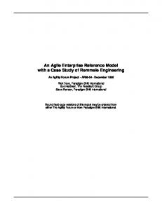
Fig. 9. (a)-(d) Example trajectories over 70 frames. Trajectory TC from tracker compared to TB - the hand marked up trajectory. The figures show the area between them, and the displacements between positions at each time step.

the floor. Figure 9 qualitatively illustrates the shifted trajectories, whilst Table 2 quantitatively highlights the systematic error present in this sequence. If TC is shifted by 500mm in the x-direction, and 600 − 700mm in the ydirection, the differences between the trajectories fall significantly. This may be due to an invalid assumption that the position of the tracked players is the midpoint of the base of the bounding box around the player. This may be due to the player’s shape in these frames, tracker error, or human mark up of the single point representing the player at each time step. Table 2. Results of trajectory evaluation. All distances are in mm.

Metric mean median min max s.d ‘area’ D(TC , TB ) 890 859 393 1607 267 326 D(TC + (510, −710), TB ) 279 256 40 67 145 133 D(TC , TB , −9) 803 785 311 1428 237 317 D(TC + (551, −618), TB , −2) 263 230 52 673 129 138

Performance Evaluation Metrics and Statistics

3.3

287

Car Tracker Example

This section compares trajectories from a car tracker [3] with manually marked up ground truth positions. In this example, the evaluation is performed in image plane coordinates (using 352 × 288 resolution images), on a sequence of cars on an inner city bypass, a sample view is shown in Figure 7.

(a) Tracked and ground truth trajectories

(b) Spatially aligned trajectories

(c) Temporally aligned trajectories

(d) Temporally and spatially aligned

Fig. 10. (a)-(d) Three pairs of example trajectories over 200 frames. Trajectory TA from tracker compared to TB - the hand marked up trajectory, with the area between them shaded.

Trajectory comparison is performed on three trajectories of cars in the scene, each over 200 frames in length. Figure 10 displays these trajectories along with the ground truth, and Table 3 details the quantitative results, from which it can be seen that there is little systematic error in the system, with each car’s centroid generally being accurate to between 1 and 3 pixels.

4

Summary and Conclusions

Quantitative evaluation of the performance of computer vision systems allows their comparison on benchmark datasets. It must be appreciated that algorithms can be evaluated in many ways, and we must not lose target of the aim of the evaluation. Here, a set of metrics for positional evaluation and comparison of trajectories has been presented. The specific aim has been to compare two trajectories. This is useful when evaluating the performance of a tracker, for quantifying

288

C.J. Needham and R.D. Boyle

the effects of algorithmic improvements. The spatio/temporally separated metrics give a useful measure for identifying the precision of a trajectory, once the systematic error is removed, which may be present due to a time lag, or constant spatial shift. There are many potential obvious uses for trajectory comparison in tracker evaluation, for example comparison of a tracker with Kalman Filtering and without [4] (clearly this affects any assumption of independence). It is also important to consider how accurate we require a computer vision system to be (this may vary between detection of a target in the scene and precise location of a targets’ features). Human mark up of ground truth data is also subjective, and there are differences between ground truth sets marked up by different individuals. If we require a system that is at least as good as a human, in this case, the tracked trajectories should be compared to how well humans can mark up the trajectories, and a statistical test performed to identify if they are significantly different. Table 3. Results of trajectory evaluation. All distances are in pixel units. Left Path Metric mean median min max s.d ‘area’ D(TA , TB ) 1.7 1.3 0.1 7.1 1.3 0.6 D(TA + (−0.2, −0.8), TB ) 1.6 1.3 0.2 6.5 1.1 0.5 D(TA , TB , 1) 1.5 1.3 0.1 5.1 0.8 0.6 D(TA + (0.8, −0.1), TB , 1) 1.3 1.2 0.1 5.2 0.8 0.5 Middle Path Metric mean median min max s.d ‘area’ D(TA , TB ) 3.0 2.3 0.4 12.4 2.2 1.8 D(TA + (1.9, −0.9), TB ) 2.3 1.9 0.1 11.2 2.0 0.9 D(TA , TB , 1) 2.9 2.3 0.5 8.7 1.4 1.8 D(TA + (3.1, 1.8), TB , 3) 1.3 1.3 0.1 3.6 0.7 0.6 Right Path Metric mean median min max s.d ‘area’ D(TA , TB ) 3.2 2.9 0.3 9.7 1.8 2.1 D(TA + (2.3, −0.2), TB ) 2.5 2.3 0.1 8.6 1.4 1.2 D(TA , TB , 0) 3.2 2.3 0.3 9.7 1.8 2.1 D(TA + (2.9, 2.0), TB , 2) 1.7 1.6 0.1 6.0 0.9 1.0

References 1. T. J. Ellis. Performance metrics and methods for tracking in surveillance. In 3rd IEEE Workshop on Performance Evaluation of Tracking and Surveillance, Copenhagen, Denmark, 2002. 2. M. Harville. Stereo person tracking with adaptive plan-view statistical templates. In Proc. ECCV Workshop on Statistical Methods in Video Processing, pages 67–72, Copenhagen, Denmark, 2002.

Performance Evaluation Metrics and Statistics

289

3. D. R. Magee. Tracking multiple vehicles using foreground, background and motion models. In Proc. ECCV Workshop on Statistical Methods in Video Processing, pages 7–12, Copenhagen, Denmark, 2002. 4. C. J. Needham and R. D. Boyle. Tracking multiple sports players through occlusion, congestion and scale. In Proc. British Machine Vision Conference, pages 93–102, Manchester, UK, 2001. 5. IEEE Workshop on Performance Evaluation of Tracking and Surveillance. http://visualsurveillance.org/PETS2000 Last accessed: 18/10/02. 6. H. Sakoe and S. Chiba. Dynamic Programming optimization for spoken word recognition. IEEE Trans. Acoustics, Speech and Signal Processing, 26(1):43–49, 1978.