Performance Evaluation of 2D Adaptive Prediction Filters ... - CiteSeerX

Performance Evaluation of 2D Adaptive Prediction Filters for Detection of Small Objects in Image Data Tarun Soni, James R. Zeidlery , and Walter H. Ku Department of Electrical and Computer Engineering University of California at San Diego, La Jolla, CA 92093-0407 yAlso with: Naval Command, Control and Ocean Surveillance Center, R.D.T. & E. Division, Code 804, San Diego, CA 92152-5000

EDICS 1.3 Abstract This paper studies the performance of two dimensional least mean square(TDLMS) adaptive lters as prewhitening lters for the detection of small objects in image data. The object of interest is assumed to have a very small spatial spread and is obscured by correlated clutter of much larger spatial extent. The correlated clutter is predicted and subtracted from the input signal, leaving components of the spatially small signal in the residual output. The receiver operating characteristics of a detection system augmented by a TDLMS prewhitening lter are plotted using Monte-Carlo techniques. It is shown that such a detector has better operating characteristics than a conventional matched lter in the presence of correlated clutter. For very low signal to background ratios, TDLMS based detection systems show a considerable reduction in the number of false alarms. The output energy in both the residual and prediction channels of such lters is shown to be dependent on the correlation length of the various components in the input signal. False alarm reduction and detection gains obtained by using this detection scheme on thermal infrared sensor data with known object positions is presented.

 This work was supported by the NSF I/UC Research Center on Ultra High Speed Integrated Circuits

and Systems (ICAS) at the University of California, San Diego, the Oce of Naval Research and the National Science Foundation under grant #ECD89-16669 and the U.S. Naval Command Control Ocean Surveillance Center, R.D.T.&E. Division's Independent Research Program.

1

1 Introduction This paper addresses the problem of detecting dim objects with very small spatial extent that are masked by spatially large clutter in image data. Applications where this is of interest include the detection of tumors and other irregularities in medical images and target detection in infrared sensor data. Prediction based methods which rely on the accuracy of speci ed image representation models are often applied to such applications [1{3]. A number of models have been proposed for clutter representation [4]. Takken et. al. [5{7] developed a spatial lter based on least mean square optimization to maximize the signal to clutter ratio for a known and xed clutter environment. A local demeaning lter has been used to track the non-stationary mean in an image by Reed et. al. in [8,9]. Chen et. al. [8] modeled the underlying clutter and noise after local demeaning as a whitened Gaussian random process and developed a constant false alarm rate detector using the generalized maximum likelihood ratio. Wang [10] and Adridges et. al. [11] use adaptive techniques to obtain a local estimate of spatially varying clutter. Other infrared systems [8, 12, 13] use multispectral data and multi-dimensional matched ltering techniques based on an underlying model of the data. One dimensional adaptive linear prediction lters have been applied to the detection of narrow band signals embedded in non-stationary noise as well as to the removal of narrow band interference from broad band data [14{18]. In the rst case a narrow band signal of interest is extracted from the prediction channel of the adaptive lter. In the second case the broad band signal of interest is extracted from the residual error of the adaptive lter [14,16]. Adaptive lters analogous to the LMS and lattice implementations in one dimension, have been recently extended to two dimensions with applications in image processing [19{23]. These algorithms update the lter weights based on the spatial coherence between the signal and noise components of the data and minimize the variance of the prediction error (residual) without explicit assumptions about the noise statistics. In this paper the performance of two dimensional least mean square (TDLMS) adaptive lters as whitening lters for the detection of signals of small spatial extent embedded in spatially distributed clutter is examined. In section 2 the TDLMS adaptive lter used in a line enhancer con guration is described. In section 3, the performance of a detection 2

system augmented by a TDLMS prewhitening lter is studied for narrowband clutter in images. The optimal weights for sinusoidal inputs are derived and the receiver operating characteristics are plotted using Monte-Carlo techniques. In section 4 the lter is applied towards the detection of point objects embedded in clouds. The reduction in false alarms due to prewhitening is described. Section 5 describes the application of the TDLMS based lter on thermal infrared multispectral (TIMS) data which contains small objects at known locations.

2 The Two Dimensional Adaptive Whitening Filter The optimal detector for known signals in stationary correlated noise is a two stage detector with the rst stage being a whitening lter [24]. For unknown and possibly nonstationary noise and clutter, an adaptive lter can be used as the rst stage whitening lter(Fig.1) as discussed in [14{16] . The Least Mean Square(LMS) algorithm can be applied as a predictor for whitening the correlated clutter in an image as shown in Fig.2. The distinction between clutter and noise in this application is based on the predictability of the two. The components of the background that are stochastic random processes will be called noise and the deterministic component of the background which are not part of the signal will be called clutter. The TDLMS adaptive lter described in [19] predicts an image pixel as a weighted average of a small window of pixels as

Y(m; n) =

NX ?1 NX ?1 l=0 k=0

Wj (l; k)X(m ? l; n ? k)

m; n = 0; : : :; M ? 1

(1)

where, X is the input image of size M  M , Y is the predicted image and Wj is the weight matrix at the j th iteration. The window size (and hence the weight matrix) is N  N . If the image is scanned lexicographically, j = mM + n. The predicted pixel value is compared with a reference image ,D(m; n), which is a shifted version of the primary image in the line enhancer con guration. The error is found as

E(m; n) = j = D(m; n) ? Y(m; n): 3

(2)

The adaptation algorithm minimizes the expected value of this mean square error over the complete image. An ideal Wiener lter implementation requires knowledge of the autocorrelation and the cross-correlation between the various regions of interest in the image and assumes stationary characteristics. Under such conditions, the ideal lter weights are then given by the two dimensional Wiener-Hopf equation as

P(l; k) =

?1 NX ?1 NX p=0 q=0

W(p; q)R(l ? p; k ? q)

l; k = 0; : : :; N ? 1

(3)

where W are the optimum lter weights, P is the crosscorrelation matrix de ned by

2 66 E. (D(m; n)X(m; n)) P = 64 .. E (D(m; n)X(m ? N + 1; n))

3 E (D(m; n)X(m; n ? N + 1)) 7 .. 77 .5 E (D(m; n)X(m ? N + 1; n ? N + 1))




.. .






and R is the input autocorrelation matrix with elements de ned by

R(l ? p; k ? q) = E (X(m ? l; n ? k)X(m ? p; n ? q)) :

(4)

In the absence of any knowledge of these statistics of the input, the LMS algorithm uses instantaneous estimates. Then, the steepest descent algorithm leads to the weight update equation

Wj+1(l; k) = Wj + j X(m ? l; n ? k)

l; k = 0; : : :; N ? 1

(5)

Separation of the clutter and signal of interest is accomplished by predicting one of them and subtracting it from the input channel. Since the image is clutter dominated, with the correlated clutter having more energy than the signal of interest, the adaptive lter is made to adapt to the clutter, and predict it. The residual or error channel then contains the signal of interest in white noise. In our implementation a causal window with quarter plane support and a left to right lexicographic scan were used, though other schemes for prediction and update can be used. For example, Ohki et. al. [20] suggest a technique for updating the lter coecients in both directions. 4

The TDLMS adaptive lter has a very low computational complexity. For a w  w sized TDLMS lter window, the computations required per pixel of the input image are O(w2) additions and O(w2) multiplications This makes it a viable choice for real time systems implementations.

3 Detection Performance for Point Objects in Narrow Band Clutter and Noise In this section we describe the performance of the two stage detection system described in section 2 for the detection of point objects in narrow band noise and clutter. The optimal lter weights of the TDLMS adaptive lter are given by the two dimensional Wiener-Hopf equation [19] as ?1 LX ?1 LX p=0 q=0

W(p; q)R(p ? l; q ? k) = P(l; k)

8 l; k 2 [0; L ? 1]

(6)

where the lter window is assumed to be L  L and the auto correlation and cross correlation matrices are given by

and

R(p ? l; q ? k) = E (X(m ? l; n ? k)X(m ? p; n ? q))

(7)

P(l; k) = E (D(m; n)X(m ? l; n ? k)) :

(8)

Here X is the primary input and D is the reference input. For the prediction lter con guration shown in Fig.2, the reference is a delayed version of the primary and hence the 2-D Wiener Hopf equation can be written as ?1 LX ?1 LX p=0 q=0

W(p; q)R(p ? l; q ? k) = R(l +
x; k +
y )

8 l; k 2 [0; L ? 1]

(9)

where (
x ;
y ) are the delays in the two directions. All the simulations in this paper were run with
x =
y = 1 which corresponds to \one step prediction". An ideal narrow band clutter in the form of a two dimensional sinusoid with random 5

phase is assumed. For such a two-dimensional sinusoid in zero mean white Gaussian noise, the autocorrelation matrix can be written as

E (X(m ? p1; n ? q1)X(m ? p2; n ? q2)) = 02(p1 ? p2 ; q1 ? q2 ) + s2cos (!x (p1 ? p2 ) + !y (q1 ? q2 ))

(10)

where 0 is the power of the white noise and s is the power of the sinusoid. To solve for the optimal weights given by Eq.9, we use the method of undetermined coecients used in [25]. For a 2-D sinusoidal input, the weights are assumed to be of the form W(p; q) = Tx Ay (11) where

h

i

Tx = ej!x p e?j!x p h i Ty = ej!y q e?j!y q

(12)

and A is the matrix of coecients as

1 0 A A 11 12 A: A=@

(13)

A21 A22

When equations 10 and 11 are applied to the 2-D Wiener-Hopf equations given by Eq.9, we get

?

e?j!x le?j!y k A2202 + A22L2 2s + A12L x 2s + A21L y 2s + A11 x y 2s ) ? +ej!x l ej!y k A1102 + A11L2 2s + A12Le?2j!y (L?1) y 2s + A21Le?2j!x (L?1) x 2s + A22 e?2j!x (L?1)e?2j!y (L?1) x y 2s ) ?
+ej!x l e?j!y k A1202 ?
+e?j!x l ej!y k A2102 2

2

2

2





s ej!x
x ej!y
y ej!x l ej!y k  2s ?j!x
x ?j!y
y  ? j! l ? j! k x y e e e 2e 2

2

2

2

=

2

2

6

where x and y are de ned by and

2j!x L

x = 11??ee2j!x

(14)

2j!y L

y = 11??ee2j!y :

(15)

On comparing the coecients of the relevant terms we get

A12 A21 ?11 A11 + A22 A11 + ?22 A22 where and

= = = =

0 0

1 ?j!x
x e?j!y
y L2 +202 =s2 e 1 j!x
x ej!y
y L2 +202 =s2 e

2j!x L ?11 = L2 + 21 2= 2 11??ee2j!x 0 s

!

1 ? e2j!y L 1 ? e2j!y

!

!

!

?2j!x L 1 ? e?2j!y L : ?22 = L2 + 21 2= 2 11??ee?2j!x 1 ? e?2j!y 0 s Now, for all ?11 ?22 6= 1 we can solve the set of equations given by Eq.16 to get

3 2 3 2 ?j!
?j!
3 2 A e x xe y y 5 ?22 ? 1 1 11 5= 4 5 4 4 ?
: (?11?22 ? 1) L2 + 202=s2 ?1 ?11 A22 ej!x
x ej!y
y

(16) (17)

(18)

Thus the weights can now be written as

W(p; q) = A11ej(!xp+!y q) + A22e?j(!x p+!y q):

(19)

Further, since ?11 = ?22 we have A11 = A22 , leading to

W(p; q) = cos (!xp + !y q + )

(20)

where  = 2 j A11 j and  = 6 A11. To con rm this analytical expression for the optimum weights a TDLMS lter with a 7

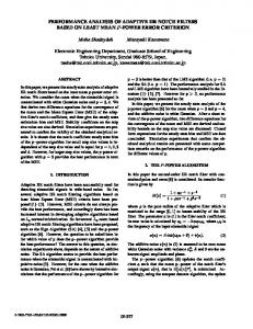
32x32 weight matrix with a  of 10?8 was applied to a two dimensional sinusoid and the weights were observed after convergence. The sinusoid was taken to have a frequency of 0.28 radians per pixel in both the axes with additive white Gaussian noise at a signal to white noise ratio of 29.59 dB. Two columns of the weight matrix are plotted in Fig.3, and the weights of the TDLMS adaptive lter agree very well with the optimum weights de ned by Eq.20. It is seen that the optimum weights are sinusoidal when the input is a stationary sinusoid. This result is similar to that obtained for a one dimensional LMS prediction lter with an input consisting of a sinusoid in white Gaussian noise [26, 27]. As in the one dimensional case, with a proper choice of , the TDLMS adaptive lter weights converge so as to predict the correlated component in the background. In [28] it is shown that the weights of a one dimensional adaptive lter can be modeled as ~ ). having two components: the optimal weights(W) and the misadjustment component(W The weights of the TDLMS can be similarly modeled with W de ned by Eq.20 and an additive misadjustment term. The prediction channel of the lter will then consist of four components: (1) The optimally predicted clutter, (2) The noise and spatially small signal of interest ltered by W, (3) the misadjustment output due to the clutter and (4) the noise ~ ). The error channel will and signal of interest ltered through the misadjustment lter (W contain components from the signal of interest and the input noise, and will also contain the misadjustment components of the clutter.

3.1 TDLMS Augmented Detection in Narrowband Noise The receiver operating characteristics of a detector augmented by a TDLMS adaptive lter were found by Monte-Carlo simulations. The infrared signal model developed by Chan et. al. [4] was used for these simulations. This model leads to a Gaussian intensity function for the object, of the form  

I (x; y) = ?e

?

?x0 )2 + (y?y0 )2

(x

x2

y2

(21)

where ? is the maximum value of the object intensity function, (x0 ; y0) is the position of the center of the object, and (x; y ) de ne the spatial spread of the object. The background,

8

C(x,y), consists of clutter and noise components of the form,

C (x; y) = aSin(!xx + !y y) + W (x; y)

(22)

where the power of the clutter component is given by a2=2 and W (x; y ) is zero mean white Gaussian noise process of variance  2. The input image then becomes

Y (x; y) = I (x; y) + C (x; y)

(23)

and is shown 1 in Fig.4a. Fig.5 shows the spectrum of the input image in the two dimensional spatial frequency domain. The sinusoidal clutter contributes to the spatial spectrum of the input with a narrowband spike at the position (!x ; !y ) of the spatial frequency space. The signal of interest is a broadband signal with its energy spread across a wide band of spatial frequencies. Fig.6 shows the two dimensional frequency domain log magnitude plot of the output image at the residual channel of the TDLMS adaptive lter. A 3  3 window with  = 1e ? 6 was used. The broadband energy of the object is seen to be present while there is a notch at the frequency of the interfering clutter, with very little energy in those frequencies. It is thus seen that the narrowband clutter has been predicted and cancelled from the input. This is also evident in Fig.4b which shows the pixel intensities of the error channel output of the TDLMS lter. The average noise energy per pixel, NE , in Fig.4a is given by 2

NE = a2 +  2:

(24)

All images in this paper are 256  256 pixels in size. They are shown with the upper left corner corresponding to the (1; 1) pixel and the lower right corner corresponding to the (256; 256) pixel. The horizontal direction corresponds to the x axis (the rst index of the image) and the vertical direction corresponds to the y axis. The intensity values for all images has been normalized to have a maximum of 255 and a minimum of 0. 1

9

The average correlation per pixel, K , in the noise can then be de ned as the ratio 2 K = a2 =a2 =+2  2 :

(25)

And the total signal energy, SE in the image is

SE =

N N X X I2(i; j ) i=1 j =1

(26)

where the image size is N  N . The signal to background ratio per pixel(PSBR) in the image then becomes PSBR = 2SE : (27)

N  NE

The Adaptive Clutter whitener(ACW) augmented detector was compared with a conventional matched lter for dierent amounts of background correlation. The lter window used was 3  3 and a  = 10?6 was chosen. The amount of correlation in the background was allowed to vary while the total NE was kept constant. Thus the PSBR was kept xed, and the correlated component (K ) in the background was increased from 0 to 1. The probability of detection and the probability of false alarm were found for both the ACW-augmented detector and the conventional matched lter and the receiver operating characteristics plotted. The probability of detection (Pd ) was found by using the detector output at the pixels where the object is known to be present and comparing it to a threshold to make a decision. 500 independent runs were used to calculate the probability of detection. The probability of false alarm (Pfa)was calculated by comparing the pixel output values of the same matched lter at pixel locations where the object was known to be absent. The threshold was selected across the range of the matched lter outputs to get dierent false alarm and detection rates. In these simulations the Pfa was found using the matched lter output at 25 random pixels in the image (suciently far away from the object location) for 500 runs giving a total of 12500 samples. A very low PSBR and consequently a very high Pfa was used to reduce the number of computations required to calculate the Pfa .

10

3.2 Operating Characteristics of the TDLMS Augmented Detector Fig.7 shows the receiver operating characteristics(ROCs) of the two detectors. When the background consists of white noise (ie, K = 0), the conventional matched lter has better operating characteristics than the augmented matched lter. This is expected, since the misadjustment in the TDLMS augmenting lter will add to the white noise in the background. Further, as K increases, the performance of both the detectors is seen to degrade and the operating characteristics move towards the right of the plot, signifying a higher Pfa for a given Pd . However, the performance of the conventional matched lter degrades much more than that of the ACW augmented lter. The operating characteristics of the conventional matched lter for a low correlation factor in the background (K = 0:11) are below those of the ACW augmented detector at K = 0:89. It should be noted that the TDLMS based ACW did not require any explicit model for the background clutter, and was able to adapt to the correlated components. The same narrow band image was also passed through a local demeaning lter using a 4  4 window. The local demeaning lter has been found to produce Gaussian image statistics [8, 9]. Further, the covariance of the output of local demeaning lters has been found to be very close to the identity matrix [8,9]. This makes the local demeaning algorithm a likely candidate for whitening lters. However, for narrow band images with a strong frequency component away from the zero frequency (in the 2-D spatial frequency domain) the local demeaning lter is not able to remove the high frequency components of the clutter. Figure 8 shows the output of the local demeaning lter. The spectrum (shown in Fig.9) of this output shows the presence of the sinusoidal clutter as the narrow band interference. If the window size of the local demeaning lter is chosen larger than 4  4, the local mean approaches the global mean and the performance of the local demeaning lter degrades.

3.3 Bounds on  The distinction between the clutter and the signal of interest is accomplished on the basis of the dierences in the correlation lengths of the signal and the background clutter. The rate of adaptation of the TDLMS lter depends very strongly on the value of the adaptation parameter . Hence, the issue of predicting only the background clutter and ignoring the 11

presence of the signal in its prediction is critically dependent on the choice of . If min and max are the largest and smallest eigenvalues of the autocorrelation matrix R de ned in Eq.4, then the number of iterations, da, required by the lter to adapt is bounded by [29] ?1 ?1 (28) ln (1 ?  )  da  ln (1 ?  ) max

min

Since the the lter weights should converge to the statistics of the noise but not to those of the signal of interest,  should be chosen such that the spatial extent of the signal, ds satis es 1 ds  ln (1 ?? (29) ) s;max

where, s;max is the largest eigenvalue of the signal \autocorrelation" matrix. Thus if  is chosen such that ?1=ds (30)   1 ? e s;max

and lies within the bounds in Eq.28, the lter will be able to predict the background clutter but not the signal of interest, and thus separate the two. It is obvious that a lower value of  will lead to more of the energy from the signal to be output in the error channel, at the same time  should high enough to converge to the background clutter statistics. Further as  is increased, the misadjustment noise increases and the lter performance will degrade. Thus it is expected that for any given set of clutter and signal correlation characteristics, there will be an optimum value of  which will give a maximum gain in the TDLMS output. This will be experimentally seen in section 5.

4 Reduction in Number of False Alarms The performance of a TDLMS prewhitening adaptive lter for nonideal backgrounds is studied in this section. To characterize the improvement obtained by the use of a TDLMS prewhitener, the false alarm rate of such a detector is used as a metric. Images consisting of single pixel signals of various intensities embedded in a cloud were generated. The cloud background was generated2 using the random midpoint displacement The program used for generating the clouds was developed by Om Sharma now at the Goddard Space Flight Center, Greenbelt, MD. 2

12

generation technique for fractals which is often used for scene generation and cloud modeling [30,31]. The correlation characteristics of such backgrounds was examined and found to be similar to the 2-D Gaussian model developed by Chan et. al. [4]. Fig.10 shows the input with 20 objects inserted at random points with random input signal to noise ratios. Fig.11 shows the output from the TDLMS ( lter window of 3  3 and  = 1e ? 7) after most of the background cloud has been cancelled and the residual output contains the signals of interest. The detectability of the signal of interest depends on the signal to background ratio in its local region and we de ne the local signal to background ratio (LSBR) as the signal to background ratio in a window around the region of interest. Thus, if the window of interest is a rectangular region de ned by (Lx ; Ly ) to (Hx; Hy ), then the LSBR (in dB) is de ned as PHx PHy (I(i; j ) ? m )2 w LSBR = 10 log10 i=Lx j=Ly2 (31) w

where, mw is the mean of the background in the window of interest and w is the variance in the same window. Since the background statistics vary across the image, the LSBR gain is not directly related to the input signal amplitude. Table 1 details the signal to background ratio gains for the 20 pixels of interest. A threshold for perfect detection can be de ned as the highest threshold at which the weakest signal of interest is detected. For this image it was found that the number of false alarms per pixel of the image, at the threshold of perfect detection, is reduced from 0.74 to 0.12 after processing with the TDLMS adaptive lter. It is thus seen that the background clutter is predicted very well by the TDLMS lter with a vast improvement in the detectability of the signals. To characterize this further, the number of false alarms for a single object in this clutter was found for varying input signal intensities, at a single location in the image with the use of a 3  3 TDLMS adaptive lter. A one pixel object was inserted at the pixel location (100,100) and detection was done by thresholding the output image to the intensity value of the object pixel at the residual output. This is the highest threshold that could be used for the detection of the inserted object. At this threshold the number of false alarms in the image were found. Fig.12 shows the change in the number of false alarms per pixel 13

of the output image as a function of the input LSBR for two dierent values of . The unprocessed image, due to the dim nature of the object and low LSBR, has a very high number of false alarms. The TDLMS whitening lter shows a vast improvement (both for the  = 10?7 and the  = 10?6 cases) with the number of false alarms in the image going to zero as the LSBR increases. As expected, the number of false alarms is less for  = 10?7 than for the  = 10?6 case, since the lower  permits better separation of the components of a signal based on their correlation lengths. The equivalent false alarm number for two dierent local demeaning lters is also shown. The local demeaning lters with window sizes of 9x9 or 7x7 show a reduction in the number of false alarms as the LSBR increases. However for very low LSBR the local demeaning lter has signi cantly high number of false alarms.

5 Performance with TIMS Sensor Data In this section we present the results obtained by applying this two stage augmented detector to infrared image data. The image used is channel 4 of a 6 channel data set collected by the NASA Thermal Infrared Multispectral Scanner(TIMS) sensor and includes a rural background over the hills of Adelaide, Australia [12]. This section includes performance data from both real and injected point objects in TIMS sensor output data. The injected objects were utilized to illustrated the performance of the TDLMS lter for known object parameters.

5.1 Dependence on the Adaptive Time Constant Fig.13 shows the behavior of 3  3 TDLMS lter as a function of  for a one pixel signal at two dierent signal intensities. As described in section 3.4, there is an optimum value of  at which the maximum gain is obtained. If  is less than this optimum value, the lter is not able to converge to the statistics of the clutter. Hence the residual channel contains some component of the correlated clutter leading to a reduced gain. If the value of  is higher than the optimum, the adaptive lter is very sensitive to changes in the input, and some of the energy from the signal of interest is also predicted and cancelled. The misadjustment noise in the adaptive lter weights increases with  and is another factor contributing to 14

the drop in gain as  increases.

5.2 Separation by Dierences in Correlation Lengths To study the ability of the TDLMS prewhitener to separate signals based on spatial correlation, simulation studies were conducted with varying signal spread. Two objects with symmetric Gaussian intensity functions de ned by Eq.21 were inserted in the infrared background. The value of  2(= x2 = y2 ) de nes the spread of the object intensity. A higher  2 leads to a more spatially spread signal. Fig.14 shows an image with the two components inserted in the background. One is the object of interest (at pixel location 100,100) which is a Gaussian shape with  2 = 2 and the other is a component of the same shape but with  2 = 98. Fig.15 shows the output of the TDLMS whitener ( lter size of 3  3 and  = 1e ? 7 ) for this case, where the component of the input with  2 = 2 is seen to be present, while the output for the  2 = 98 case is absent. Figure 16 shows the energy at the pixel of interest in the residual channel output of the TDLMS lter as a function of the signal correlation length ( 2). An object de ned by Eq.21 was used and the pixel intensity at the output observed. It is seen that as the correlation length increases, the output energy at the pixel of interest decreases. Further, as shown in Fig.17, the energy in the prediction channel of the TDLMS lter correspondingly increases as the correlation length increases. It should be noted that the prediction channel output always contains the energy due to the non zero mean of the image which is seen in Fig.17 as a base level of 1:3  104. In both these plots, three regions (depending on  ) can be de ned for this TDLMS adaptive lter:

 (1) For objects with very small correlation length, the energy is contained almost totally in the output channel.

 (2) For objects of long correlation length, the energy is absent from the output.  (3) For objects of intermediate correlation length, there is a partial decorrelation between the input and reference channels. In such cases the energy of the object is split between both channels. 15

A similar plot for the local demeaning lter is shown in Fig.18, and it is seen that the local demeaning lter is not able to provide a clear boundary between the two regions of diering correlation spread. Thus we see that the TDLMS is able to separate the object of interest from the clutter based on their correlation spread.

5.3 Detection of Small Objects in Spatially Correlated Clutter In [12] Ho et. al. identi ed 14 pixels which contained small objects in the TIMS sensor data described above. The 14 pixels were identi ed on the basis of multispectral data in the 6 separate bands. The locations designated in [12] are illustrated in by boxes in Fig.19. The pixel intensities at the output of the TDLMS lter (residual channel) is shown in Fig.20. A 3  3 TDLMS lter with  = 10?7 was used. Table 6 describes the input and output signal to background ratios for these pixels. Note that the gain is very nonuniform across the image. This is a result of variations in the LSBR across the image. Fig.21 shows a high resolution intensity plot around the 13th object de ned in Table 6. As seen in the gure and described in the table, this object has a very high LSBR. This causes the object to be predicted. Fig.22 shows the corresponding output for this pixel. It is seen that there are a number of pixels in the local region with comparable intensity. Fig.23 is a similar high resolution plot around the 14th object de ned in Table 6. In this case, due to the low LSBR, the output (shown in Fig.24) is seen to contain energy due to the object pixel and there is a vast improvement in the detectability. This is also seen in the LSBR gain for this pixel as seen in Table 6. Though there is a loss in LSBR at some pixels it is seen that the detection performance of the lter improves considerably when the input image is processed by the TDLMS adaptive lter. For a threshold set to detect all 14 of the signal mentioned in Table 6, the number of false alarms in the image is signi cantly reduced. If the detection criterion is changed to reduce the number of detected objects the number of false alarms in the image are further reduced. A plot of the percentage of objects detected as a function of the number of false alarms per pixel is shown in Fig.25. A similar plot for the local demeaning lter is also shown in this gure and it is seen that for a xed number of false alarms per pixel the percentage of of objects detected is much higher when the data is processed with the TDLMS based adaptive lter than with the local demeaning lter. 16

6 Conclusions The TDLMS adaptive prediction lter was applied to the problem of detecting objects in image data. It is seen that for correlated inputs, the TDLMS lter weights converge to the solution of the two dimensional Wiener-Hopf equation. This leads to the clutter in the image being predicted thereby allowing the signal of interest to be enhanced relative to the background clutter. For an ideal two dimensional sinusoidal input as clutter, the lters weights were shown to be sinusoidal, analogous to the one dimensional lter. It was shown that the TDLMS based lter creates a notch in the spatial frequencies of the narrow band clutter. On simulated cloud data and in TIMS sensor data containing small objects at known locations, it was also shown that the number of false alarms is signi cantly reduced when the input is preprocessed with the TDLMS lter. The separation of the signal of interest from the clutter was seen to depend on the energy of the signal and the dierence in correlation length between the background and the object of interest. It is seen that the gain obtained by prewhitening depends on the local correlation characteristics of the image around the pixel of interest.

References [1] C. W. Therrien, T. F. Quatieri, and D. E. Dudgeon, \Statistical Model-Based Algorithms for Image Analysis," Proceedings of the IEEE, vol. 74, pp. 532{551, Apr. 1986. [2] A. K. Jain, Fundamentals of Digital Image Processing. Englewood Clis, NJ.: Prentice Hall, 1989. [3] A. K. Jain, \Advances in Mathematical Models for Image Processing," Proceedings of the IEEE, vol. 69, pp. 502{528, 1981. [4] D. S. K. Chan, D. A. Langan, and D. A. Staver, \Spatial Processing Techniques for the Detection of Small Targets in IR Clutter," in Proc. of SPIE, Technical Symposium on Optical Engineering and Photonics in Aerospace Sensing, (Orlando, Florida), Apr.,1990. 17

[5] R. Nitzberg, E. H. Takken, D. Friedman, and A. F. Milton, \Spatial Filtering Techniques for IR Sensors," in Proc. of SPIE, Technical Symposium on Smart Sensors, vol. 178, 1979. [6] E. H. Takken, D. Friedman, A. F. Milton, and R. Nitzberg, \Least-mean-square Spatial Filter for IR Sensors," Applied Optics, vol. 18, no. 24, pp. 4210{4222, 1979. [7] M. S. Longmire and E. H. Takken, \LMS and Matched Digital Filters for Optical Clutter Suppression," Applied Optics, vol. 27, no. 6, pp. 1141{1159, 1988. [8] J. Y. Chen and I. S. Reed, \A Detection Algorithm for Optical Targets in Clutter," IEEE Transactions on Aerospace and Electronic Systems, vol. 23, no. 1, pp. 46{59, 1987. [9] A. Margalit, L. S. Reed, and R. M. Gagliardi, \Adaptive Optical Target Detection Using Correlated Images," IEEE Transactions on Aerospace and Electronic Systems, vol. 21, pp. 394{405, May 1985. [10] D. Wang, \Adpative Spatial/Temporal/Spectral Filters for Background Clutter Suppression and Target Detection," Optical Engineering, vol. 21, pp. 1033{1038, Dec. 1982. [11] A. Adridges, G. Cook, S. Mansur, and K. Zonca, \Correlated Background Adaptive Clutter Suppression and Normalisation Techniques," in Proc. of SPIE, Multispectral Image processing and Enhancement, vol. 933, 1988. [12] L. E. Ho, J. R. Evans, and L. E. Bunney, \Detection of Targets in Terrain Clutter by Using Multispectral Infrared Image Processing," Technical Report for Naval Ocean Systems Center, Dec. 1990. [13] H. Wang and L. Cai, \On Adaptive Multiband Signal Detection with the SMI Algorithm," IEEE Transactions on Aerospace and Electronic Systems, vol. 26, pp. 768{773, May 1990. [14] J. R. Zeidler, \Performance analysis of LMS Adaptive Prediction lters," Proceedings of the IEEE, vol. 78, pp. 1781{1806, Dec. 1990. 18

[15] J. T. Rickard, J. R. Zeidler, M. J. Dentino, and M. Shensa, \A Performance Analysis of Adaptive Line Enhancer-Augmented Spectral Detectors," IEEE Transactions on Acoustics, Speech, and Signal Processing, vol. ASSP-29, pp. 694{701, June 1981. [16] L. Milstein, \Interference Rejection Techniques in Spread Spectrum Communications," Proceedings of the IEEE, vol. 76, pp. 657{671, June 1988. [17] G. A. Clark and P. W. Rodgers, \Adaptive Prediction Applied to Seismic Event Detection," Proceedings of the IEEE, vol. 69, pp. 1166{1168, Sep. 1981. [18] N. Ahmed, R. J. Fogler, D. L. Soldan, G. R. Elliott, and N. A. Bourgeois, \On An Intrusion Detection Approach Via Adaptive Prediction," IEEE Transactions on Aerospace and Electronic Systems, vol. 15, pp. 430{437, May 1979. [19] M. M. Hadhoud and D. W. Thomas, \The Two-Dimensional Adaptive LMS(TDLMS) Algorithm," IEEE Transactions on Circuits and Systems, vol. 35, no. 5, pp. 485{494, 1988. [20] M. Ohki and S. Hashiguchi, \Two-Dimensional LMS Adaptive Filters," IEEE Transactions on Consumer Electronics, vol. 37, pp. 66{73, Feb. 1991. [21] M. Ohki and S. Hashiguchi, \A New 2-D LMS Adaptive Algorithm," in Proceedings IEEE International Conf. on Acoustics Speech and Signal Processing, vol. 4, (Toronto, Canada), pp. 2113{2116, April 1991. [22] H. Youlal, M. Janati-i, and M. Najim, \Two-Dimensional Joint Process Lattice For Adaptive Restoration of Images," To be Published in the IEEE Transactions on Image Processing, July 1992. [23] W. B. Mikhael and S. M. Ghosh, \Two-Dimensional Block Adaptive Filtering Algorithms," in Proceedings IEEE International Symposium on Circuits and Systems, no. 3, pp. 1219{1222, May 1992. [24] A. Whalen, Detection of Signals in Noise. New York: Academic Press, 1971.

19

[25] J. R. Zeidler, E. H. Satorius, D. M. Chabries, and H. T. Wexler, \Adaptive Enhancement of Multiple Sinusoids in Uncorrelated Noise," IEEE Transactions on Acoustics, Speech, and Signal Processing, vol. ASSP-26, pp. 240{254, June 1978. [26] A. Nehorai and M. Morf, \Enhancement of Sinusoids in Colored Noise and the Whitening Performance of Exact Least Squares Predictors," IEEE Transactions on Acoustics, Speech, and Signal Processing, vol. ASSP-30, pp. 353{363, June 1982. [27] C. M. Anderson, E. H. Satorius, and J. R. Zeidler, \Adaptive Enhancement of Finite Bandwidth Signals in White Gaussian Noise," IEEE Transactions on Acoustics, Speech, and Signal Processing, vol. 31, pp. 17{28, Feb. 1983. [28] J. T. Rickard and J. R. Zeidler, \Second Order Output Statistics of the Adaptive Line Enhancer," IEEE Transactions on Acoustics, Speech, and Signal Processing, vol. ASSP27, pp. 31{39, Feb. 1979. [29] S. Haykin, Adaptive Filter Theory. Englewood Clis, NJ: Prentice-Hall, 1985. [30] B. B. Mandelbrot, The Fractal Geometry of Nature. New York: W. H. Freeman and Co., 1982. [31] H. O. Peitgen and D. Soupe, The Science of Fractal Images. New York: SpringerVerlag, 1988.

20

gures/twostage.ps

Figure 1: A Two Stage Filtering and Detection Procedure.

21

gures/twodale.ps

Figure 2: A Two Dimensional Adaptive Filter.

22

x10 -3 2

o o o

* * *

1.5

*

*

o *

* * * *

o

o o

*

1

*

* * o

* o

* o *

6

* o

*

mn 1

0.5 0

o

Colu

o * o

*

o

-0.5

o

o o

Colu

-1

-2 0

o

*

o

Column 1 Theory o Simulation

o

*

o o o

*

*

o

-1.5

Column 16 Theory * Simulation

*

mn 1

Weight Value

o *

* *

o

* *

5

10

15

o

o o

*

20

o

o

25

30

35

40

Row Number

Figure 3: Two columns of the weight matrix : The simulation was done with a 32x32 TDLMS lter with  = 1e ? 8 and the weights after

convergence are seen to agree with the theoretical expression.

23

(a) Input

at LSBR=9.41dB

24

Output from the residual channel of the TDLMS Filter: LSBR = 27.18dB (b)

Figure 4: Sinusoidal Clutter with small object signal at (115,45) with K = 1 25

Relative Magnitude in dB

10 0 10 -20 10 -40 10 -60 10 -80

0

2π

x fr

equ

enc

y 2π 0

ency

u y freq

Figure 5: Spatial 2-D FFT of the signal in Sinusoidal Clutter

(Log Magnitude Plot).

26

Relative Magnitude in dB

10 0 10 -20 10 -40 10 -60

0

2π

x fr

equ

enc

y 2π

ency

0

u y freq

Figure 6: Spatial 2-D FFT of the Output (Residual) of the TDLMS lter

(Log Magnitude Plot).

27

1 ACW Augmented MF

Probability of Detection

Conventional MF K = 0.66 K = 0.11 K = 0.11 K = 0.82 K K == 0.89 0.89

K = 0.33

0.1 0.01

0.1 Probability of False Alarm

1

Figure 7: The Operating Characteristics of a detector augmented by an

Adaptive Clutter Whitener at PSBR = -27.55 dB.

28

Figure 8: The Output of a 4x4 local demeaning lter LSBR = 10.78dB

(Signal of interest is at (115,45)) .

Relative Magnitude in dB

10 0 10 -20 10 -40 10 -60 10 -80 10 -100 10 -120

0

2π

x fr

equ

enc

y 2π

ency

0

u y freq

Figure 9: Spatial 2-D FFT of the Local Demeaning Filter Output

(Log Magnitude Plot).

29

Figure 10: Cloud with 20 signals inserted at random:

Input to TDLMS Filter.

Figure 11: Cloud with 20 signals: Output Energy in TDLMS Filter Resid-

ual.

30

Location LSBR in (dB) LSBR Gain x 83 152 160 128 55 129 51 60 153 190 129 148 155 164 57 99 163 105 197 163

y 57 152 108 175 58 151 108 113 138 177 64 112 187 89 160 145 199 87 158 148

Input 5.126 2.611 5.257 6.972 6.064 -3.853 4.046 8.405 7.852 5.559 12.235 5.051 6.469 12.225 9.217 12.999 9.671 10.116 13.152 10.744

Output 14.185 13.803 17.453 16.336 14.225 -2.696 18.604 14.866 19.242 12.718 16.990 18.667 18.502 18.894 16.128 17.179 17.199 16.872 19.159 14.434

in dB 9.059 11.192 12.196 9.364 8.161 1.157 14.558 6.461 11.390 7.159 4.755 13.616 12.033 6.669 6.911 4.18 7.528 6.756 6.007 3.69

Table 1: 20 Randomly inserted signals into the cloud image, with the input and output statistics ( = 10?7).

31

10 0

Number of False Alarms per pixel at the output

o

o +

10 -1 +

o

o

o

+ +

+ +

+ +

o + +

o

+ +

10 -2

Unprocessed Image

o o o o o o o o o o o ooooo

o

o o o

o

o

o o o o oo o

+ + + + + + + + + ++ Local Demeaning + + ++ + + ++ + W=9x9 ++ + ++ +++ ++ ++ W=7x7 +

10 -3

+ + + *

*

*

*

*

*

10 -4

+ +

* * * * * ** *** * ***** *

µ =1e-6

* *

+ +

+ + + + + + + ++

*

TDLMS Prewhitening µ =1e-7

*

10 -5

0 False Alarms 10 -6 -30

*

-25

*

-20

*

* * * * * * * * * * ******

-15

-10

* * *

-5

*

0

*

* * * * * **

5

10

Input LSBR in dB

Figure 12: Cloud with single object at (100,100). False detections per

pixel in the image, for perfect detection as the signal LSBR changes.

32

*

25

*

*

*

* *

* * *

* *

LSBR Gain in dB

20

*

Input LSBR = -13.9dB

*

15

Bound on o

10

o

o

*

o

o

o

µ

o

o o o

o

Input LSBR = 3.9dB

o

5

o

0 10 -10

o

10 -9

10 -8

10 -7

10 -6

10 -5

10 -4

Adaptation Constant µ

Figure 13: Gain vs.  for the Adelaide background with one pixel signal

at (100,100).

33

Figure 14: Signal with two components: object of interest at (100,100) with correlation spread of 2 = 2 and spurious component at (200,200) with correlation spread of 2 = 98.

Figure 15: The residual channel output for Fig.15. TDLMS was used with a 3x3 window and  = 1e ? 7. LSBR at (100,100) = 16.024dB

and LSBR at (200,200) = -16.75dB. 34

Energy in target pixel of Residual

10000

8000 µ =5e-8 6000 µ =1e-7 µ =5e-7 4000 µ =1e-6 2000

0 0 10

1

2

10 Correlation Length σ 2

10

Figure 16: Energy at the pixel of interest in the output of the TDLMS as

a function of the correlation length.

x10 4 6 o

*

o

Energy in target pixel of predicted image

o

o

5.5 µ =1e-6

5

* *

*

4.5

µ =5e-7

o

µ =1e-7

*

o *

+ x

+ x

+ x

o * + x

+ x + x

4 3.5 + x

µ =5e-8

3

o

2.5

* + x

2 1.5 1 10 0

o x + *

10 1 Correlation Length σ

10 2 2

Figure 17: Energy at the pixel of interest in the prediction channel of the

TDLMS as a function of the correlation length. 35

x10 7

Intensity at target pixel in Local Demeaning Output

16 14 12 +

W=9x9

10 8

W=7x7

*

W=5x5

6 4

o +

2 *

0 10 0

o

+ * o

+ o *

10 1

+ o *

+ o *

+ o *

10 2

Correlation Length σ

+ o *

+ o *

10 3

2

Figure 18: Energy at the pixel of interest in the output of the Local De-

meaning lter as a function of the correlation length.

36

Figure 19: The infrared image data with the 14 pixels of interest. Note

that some objects are clustered close to each other their enclosing boxes overlap.

Figure 20: The infrared image data output from TDLMS adaptive ter

for Fig.20.

37

Location Signal Background LSBR in (dB) LSBR Gain x y Energy Energy Input Output in dB 133 133 137 137 162 163 57 58 237 237 245 246 199 188

50 51 76 77 51 50 194 195 66 67 158 158 92 235

594 0.4414 13.453 2187 2103 934 52.3 10386 11.31 836 124 88.06 10406 65.5

501.97 493.27 334.868 342.05 367.06 405.636 553.56 710.61 714.05 721.38 293.53 315.05 664.67 864.01

0.7291 -30.4829 -13.9606 8.0567 7.5810 3.6219 -10.2467 11.6483 -18.0020 0.6414 -3.7509 -5.5360 11.9468 -11.2025

12.6507 11.8246 13.5457 16.6005 7.7111 9.6000 13.0149 10.7177 13.4291 8.2041 1.4168 8.0799 -6.6192 7.3820

11.9216 42.3074 27.5063 8.5438 0.1302 5.9781 23.2616 -0.9306 31.4310 7.5627 5.1678 13.6158 -18.5659 18.5845

Table 2: The input and output statistics of pixels declared as objects of interest in the Adelaide image data ( = 10?7).

38

Intensity

252

65 0 33 x 33

y 0

Figure 21: High resolution intensity plot of a 33x33 window around the

pixel (199,92) before processing.

Intensity

5735

0 0 33 x 33

y 0

Figure 22: High resolution intensity plot of a 33x33 window around the

pixel (199,92) after processing. 39

Intensity

241

76 0 33 x 33

y 0

Figure 23: High resolution intensity plot of a 33x33 window around the

pixel (188,235) before processing.

Intensity

15558

0 0 33 x 33

y 0

Figure 24: High resolution intensity plot of a 33x33 window around the

pixel (188,235) after processing. 40

1

o o

0.9 0.8

Percentage of Targets Detected

*+

o

TDLMS Prewhitening

+ *

o

+ *

o

0.7

+

*

o

+

*

Local Demeaning

0.6

o

0.5

0 10 -6

10 -5

+

*

o* +

+

*

o

o

+

*

o

0.2

+

*

o

0.3

+

*

o

Unprocessed

+

*

o

0.4

0.1

*+

+

*

10 -4

10 -3

10 -2

10 -1

10 0

False Alarms per pixel

Figure 25: False alarms in the Adelaide image for known objects as the

percentage of objects detected is lowered. TDLMS was used with  = 1e ? 7.

41

List of Figures 1 2 3 4 5 6 7 8 9 10 11 12 13 14 15 16

A Two Stage Filtering and Detection Procedure. : : : : : : : : : : : A Two Dimensional Adaptive Filter. : : : : : : : : : : : : : : : : : : : Two columns of the weight matrix : The simulation was done with a 32x32 TDLMS lter with  = 1e ? 8 and the weights after convergence are seen to agree very well with the theoretical expression. Sinusoidal Clutter with small object signal at (115,45) with K = 1 Spatial 2-D FFT of the Signal in Sinusoidal Clutter (Log Magnitude Plot) : : : : : : : : : : : : : : : : : : : : : : : : : : : : : : : : : : : : : : : Spatial 2-D FFT of the Output (Residual) of the TDLMS lter (Log Magnitude Plot) : : : : : : : : : : : : : : : : : : : : : : : : : : : : The Operating Characteristics of a detector augmented by an Adaptive Clutter Whitener at PSCR = -27.55 dB : : : : : : : : : : : : : The Output of a 4x4 local demeaning lter LSBR = 10.78dB : : : Spatial 2-D FFT of the Local Demeaning Filter Output (Log Magnitude Plot) : : : : : : : : : : : : : : : : : : : : : : : : : : : : : : : : : : Cloud with 20 signals inserted at random: Input to TDLMS Filter Cloud with 20 signals: Output Energy in TDLMS Filter Residual Cloud with single object at (100,100). False detections per pixel in the image, for perfect detection, as the signal LSBR changes. : Gain vs.  for the Adelaide background with one pixel signal at (100,100). : : : : : : : : : : : : : : : : : : : : : : : : : : : : : : : : : : : : Signal with two components: object of interest at (100,100) with correlation spread of 2 = 2 (LSBR=14.98dB) and spurious component at (200,200) with correlation spread of 2 = 98(LSBR=6.86dB) The residual channel output for Fig.15 TDLMS was used with a 3x3 window and  = 1e ? 6 LSBR at (100,100) = 16.024dB and LSBR at (200,200) = -16.75dB. : : : : : : : : : : : : : : : : : : : : : : Energy at the pixel of interest in the output of the TDLMS as a function of the correlation length : : : : : : : : : : : : : : : : : : : : : 42

21 22 23 25 26 27 28 29 29 30 30 32 33 34 34 35

17 Energy at the pixel of interest in the prediction channel of the 18 19 20 21 22 23 24 25

TDLMS as a function of the correlation length : : : : : : : : : : : : Energy at the pixel of interest in the output of the Local Demeaning lter as a function of the correlation length : : : : : : : : : : : : : : Infrared image data with the 14 pixels of interest. Note that some objects are clustered close to each other and hence their enclosing boxes overlap. : : : : : : : : : : : : : : : : : : : : : : : : : : : : : : : : : Infrared image data output from TDLMS adaptive ter with the 14 pixels of interest. : : : : : : : : : : : : : : : : : : : : : : : : : : : : : High resolution intensity plot of a 33x33 window around the pixel (199,92) before processing. : : : : : : : : : : : : : : : : : : : : : : : : : High resolution intensity plot of a 33x33 window around the pixel (199,92) after processing. : : : : : : : : : : : : : : : : : : : : : : : : : : High resolution intensity plot of a 33x33 window around the pixel (188,235) before processing. : : : : : : : : : : : : : : : : : : : : : : : : : High resolution intensity plot of a 33x33 window around the pixel (188,235) after processing. : : : : : : : : : : : : : : : : : : : : : : : : : : False alarms in the Adelaide image for known objects as the percentage of objects to be detected is allowed to lowered. : : : : : :

43

35 36 37 37 39 39 40 40 41