performance evaluation of conceptual and physically based ...

PERFORMANCE EVALUATION OF CONCEPTUAL AND PHYSICALLY BASED HYDROLOGIC MODELS E. A. Meselhe*, E. H. Habib University of Louisiana at Lafayette Lafayette, LA, 70504 F.L. Ogden University of Connecticut Storrs, CT, 06269-2037 ABSTRACT

the advantage of simulating complex hydrologic systems and utilizing distributed field hydrologic data. It is also recognized that, compared to conceptual lumped models, physically based distributed models are more complex to setup, have more stringent data requirements, and can be subject to over-parameterization. However, the increasing availability of distributed data on rainfall and watershed properties, along with the exponential improvement in computational resources, have increased the interest of both research and applied communities in the development and applications of such models.

This paper focuses on evaluating the performance of physically based distributed and conceptual models, and assesses their sensitivity to changes in the temporal and spatial sampling of rainfall. The Hydrologic Modeling System (HMS) was selected to represent conceptual hydrologic models, while MIKE-SHE and GSSHA were selected to represent distributed physically based models, This manuscript presents results with MIKE-SHE, while the poster at the conference will include results from GSSHA. The performance evaluation criterion is the overall agreement between observed and predicted hydrographs and the models' ability to predict time and magnitude of peak discharges and runoff volume. Both models were carefully calibrated and validated using numerous storm events for a 21.4 km2 watershed in northern Mississippi. The results indicated that MIKESHE captured the peak runoff discharges and total runoff volume better than HMS. However, overall, the performance of both models was quite reasonable. To assess the models' requirements for rainfall information, an in-depth investigation of the impact of the spatial and temporal sampling of rainfall on the prediction accuracy of each model was conducted. The study showed that MIKE-SHE was more sensitive to both the spatial and temporal sampling of rainfall than HMS.

Recent advances in the development of both conceptual and physically based models have lead to a number of model inter-comparison and evaluation studies. A detailed discussion of such studies is given in Michaud and Sorooshian (1994a), Refsgaard and Knudsen (1996), and Perrin et al., (2001). A review of these comparative studies indicates that the performance accuracy of the two modeling approaches varies widely. The comparable performance accuracy obtained with three models of varying degrees of complexity lead Refsgaard and Knudsen (1996) to recommend the use of conceptual models especially when calibration data is available, and to limit the use of complex physically based data for ungauged basins where they are expected to have a better performance. As discussed by Refsgaard and Knudsen (1996), the superiority of complex physically based 1. INTRODUCTION models over simpler conceptual models remains at the hypothesis level and has not been unambiguously asntbnuamiosy hyoesslvlad Currently available watershed models range from Currleconctualy availablemwed models to praengve fsupported by actual and sufficient performance evaluation simple conceptual lumped models to comprehensive tests. Recently, the Hydrology Laboratory of the National physically based distributed models. Conceptual lumped Weather Service (NWS) office of hydrology has models use an integrated description of parameters conducted an extensive model inter-comparison study to representing an average value over the entire catchment. assess the performance of several physically based A watershed can be divided into a number of submodels against operational lumped models (Smith et al., catchments where the hydrologic parameters may vary 2004; Reed et al., 2004). The study found that, in more from one sub-catchment to another. In such case, lumped cases, the lumped model outperformed the distributed models may be labeled as "semi-distributed." They models. However, the NWS study indicated a wide range remain non-physically based, however, as they use of accuracies among model results and suggested that synthetic methods of transforming rainfall to runoff. factors such as model formulation and the modeler's skill can have bigger impact than the type of the used model. The present study builds on the continuous research efforts to investigate the capabilities and limitations of conceptual versus physically based models. Specifically, the study evaluates the prediction accuracy of two

Distributed physically based models, on the other hand, can account for spatial variations in input parameters and state variables within the catchment. They incorporate physical formulations of the different hydrologic processes. Therefore, this class of models has

1

Report Documentation Page

FormApproved OMB No. 0704-0188

Public reporting burden for the collection of information is estimated to average 1 hour per response, including the time for reviewing instructions, searching existing data sources, gathering and maintaining the data needed, and completing and reviewing the collection of information. Send comments regarding this burden estimate or any other aspect of this collection of information, including suggestions for reducing this burden, to Washington Headquarters Services, Directorate for Information Operations and Reports, 1215 Jefferson Davis Highway, Suite 1204, Arlington VA 22202-4302. Respondents should be aware that notwithstanding any other provision of law, no person shall be subject to a penalty for failing to comply with a collection of information if it does not display a currently valid OMB control number. 1. REPORT DATE

00

2. REPORT TYPE

DEC 2004

3. DATES COVERED

N/A

4. TITLE AND SUBTITLE

5a. CONTRACT NUMBER

Performance Evaluation Of Conceptual And Physically Based Hydrologic

5b.

GRANT NUMBER

Models 5c. PROGRAM ELEMENT NUMBER 6. AUTHOR(S)

5d. PROJECT NUMBER 5e. TASK NUMBER 5f. WORK UNIT NUMBER

7. PERFORMING ORGANIZATION NAME(S) AND ADDRESS(ES)

8. PERFORMING ORGANIZATION

University of Louisiana at Lafayette Lafayette, LA, 70504; University of Connecticut Storrs, CT, 06269-2037

REPORT NUMBER

9. SPONSORING/MONITORING AGENCY NAME(S) AND ADDRESS(ES)

10. SPONSOR/MONITOR'S ACRONYM(S) 11. SPONSOR/MONITOR'S REPORT NUMBER(S)

12. DISTRIBUTION/AVAILABILITY STATEMENT

Approved for public release, distribution unlimited 13. SUPPLEMENTARY NOTES

See also ADM001736, Proceedings for the Army Science Conference (24th) Held on 29 November - 2 December 2005 in Orlando, Florida., The original document contains color images. 14. ABSTRACT 15. SUBJECT TERMS 16. SECURITY CLASSIFICATION OF: a. REPORT

b. ABSTRACT

c. THIS PAGE

unclassified

unclassified

unclassified

17. LIMITATION OF

18. NUMBER

ABSTRACT

OF PAGES

UU

8

19a. NAME OF RESPONSIBLE PERSON

Standard Form 298 (Rev. 8-98) Pirscribed by ANSI StdZ39-18

different rainfall-runoff models, conceptual semidistributed and physically based distributed models, focusing on the sensitivity of both modeling approaches to the quality and accuracy of the rainfall information. It has been a common belief by the hydrologic community that rainfall variability, both in space and time, has a significant on the response hydrologicthesystems. Therefore, aeffect number of studies haveofaddressed impact~iof rainfall sampling resolution on the prediction accuracy of hydrologic models, m e ax and somewhat mixed results were often reported. Wilson et al. (1979), Krajewski et al. (1991), Ogden and Julien (1993), Holman-Dodds et al. (1999), and Michaud and Sorooshian (1994b), have shown that the variability and the sampling resolution of rainfall can have a significant influence on the results of Other studies by Beven and hydrologic models. et al. (1994), however, have Obled and (1982) Hiomberger

while the soil can be classified into two main types: Silt loam (80%) and clay loam (20%) (Blackmarr, 1995).

/

4

J•

•

•

55*

2 11 1

l0

0

shown that a correct estimation of the total rainfall volume is more important for accurate flow prediction than providing the model with detailed spatial and temporal patterns.

"

1

2

ecale • Rain Gage

Kilometes

Q Streamfiew Gage

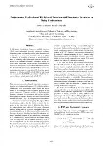
Figure 1: Location of the monitoring stations in the Goodwin Creek watershed. 3. MODEL CALIBRATION AND VALIDATION

The present study has two main objectives: (1) To compare the performance accuracy of two different hydrologic models, conceptual and physically based, and (2) to investigate the relative sensitivity of both modeling approaches to the sampling resolution of rainfall.

Both models, MIKE-SHE and HMS, were calibrated and validated using the split-sample test method as described by Klemes (1986). Accordingly, one set of data was used to calibrate the models while another of data were reserved for model validation. During the calibration procedure, physical and numerical parameters, such as loss and routing coefficients were adjusted and fine-tuned to minimize the difference between the model results and the field observations. However, parameter adjustments remained within the physically acceptable ranges based on information available in the literature. It should be noted that both models were calibrated using the runoff discharge measured at the outlet of each subbasin within the watershed.

2. THE STUDY SITE The Goodwin Creek experimental watershed located at the north central part of Mississippi was selected for this study. The National Sediment Laboratory of the United States Department of Agriculture in Oxford Mississippi has been monitoring the watershed since 1981. Detailed information about the watershed and the available data can be found in Alonso and Binger (2000).

Afterwards, a second independent set of data was used to validate the models. No further adjustments to the parameters were allowed at this stage, and the land use and other watershed characteristics were assumed to remain unchanged.

The watershed has a fairly steep topography with drainage area of 21.4 km2. The terrain elevation in the watershed, with reference to mean sea level, ranges from 71 m near the outlet to 128 at the catchment divide with an average channel slope of 0.004. It has a humid climate (hot in summer and warm in winter), an average annual temperature of about 65oF, an average annual rainfall of about 1440.2 mm (56.7 inches), and a mean annual runoff of 144.8 mm (5.7 inches).

4. EVALUATION CRITERIA The criteria used to evaluate the performance of the models are the overall agreement between predicted and measured runoff discharges, and the models' ability to predict time and magnitude of hydrograph peaks, and runoff volume. The following statistical measures were used to quantify the performance accuracy of both models during each simulation periods, and combined over all periods:

A network of 30 gauges is used to measure precipitation over the watershed. The watershed has been divided into 14 sub-catchments with a flow-recording flume constructed at the outlet of each. Figure 1 shows a map of Goodwin Creek watershed along with the locations of the monitoring stations. The land-use in the watershed can be described as follows: idle land and pasture (60%), forest (26%) and cultivated land (14%),

2

(1) Absolute Runoff Volume Error V.= Vp

-

(l-a)

V,

ev-yr

Where, Pe is relative peak error (%), Pp is the predicted Peak Flow (m3/s), Pr is the reference peak flow (m3/s), i is the peak counter, and N is the number of Peaks.

(1-b)

x 100

-

(4) Error in Peak Time

Where, Ve is the runoff volume error (m3 or %), Vr is

N

the reference runoff volume (m3), and Vp is the predicted

L.

runoff volume (m3).

T.

Runoff2

- Qni

I(Qpi

2 __input

N RMSE =

(6)

CALIBRATION AND VALIDATION RESULTS

pi- aJ i=1

N N(6

(2-a)

N= N(5. -

N

Tpi-i

Where Te is the error in peak time (minutes), Tp is the predicted peak time, Tr is the reference peak time, and N is the number of peaks. The reference quantities used in the above statistics will be clearly defined in the upcoming sections.

(2) Root Mean Square Error

RMSE =

T

x l00

-

(2-b)

Qr

It is important to state that the raw precipitation data were aggregated to 15 minutes accumulations and used as to both models. Figures 2 through 4 and Table 1 show a summary of the models performance. The statistics shown in Table 1 are based on the all the validation periods combined together.

Where, Qp is the predicted Flow (m3/s), Qr is the reference flow (m3/s), Qr is the mean flow of reference (m3/s), i is the hourly counter, and N is the number of discharge observed-predicted pairs. Rainfall:

3-

Obsoved MIs-••E M

2520-

-0

S

15 10-

N2 A

RMSE =

-

Rr)

5

100

Nx

(3)

r,

RAti

4/20/82

Figure 2: Measured and simulated discharge at the

Where, Rri is the rainfall intensity a reference sampling frequency,

4/19/82

catchment outlet (calibration period).

is the aggregated intensity at

sampling frequency of At (30-minute, 1-hr, 2-hr, etc.). (3) Relative Peak Error 1

S'--

Simple Average:

x100

PJ =

(4)

N N

"I P, i •1P00 Weighted Average: Pe =

P i=1

P

xOOxP

Figure 3: Measured and simulated discharge at the (

N

i=1

(5)

catchment outlet (validation periods).

Table 1: Statistical Summary of the Models Performance Volume Error ..

(m )

RMSE

Relative Peak Error Peak Time % Error Simple Weighted (min)

%.

m3Is I %.

3.1 5.9

2.5 6.8

18.0 30.2

15.0

11.9

30.3

25.5

19.1

24.6

_Calibration

MIKE-SHE HIvMS

-28,766 33,213

-1.8 2.1

MIKE-SHE

726,370

4.9

1.17 48.3 1.7 68.4 Validation 1.9 63.6

HIMS

1,116,109

7.5

2.1

69.9

also comparable to experiments performed by Shah et al. (1996) where a simple lumped and distributed models performed well under wet antecedent moisture conditions.

6. RAINFALL TEMPORAL SAMPLING ANALYSIS This experiment was designed to study the sensitivity of the models to changes in the temporal sampling of precipitation data. The 15-minute rainfall data were aggregated into 30-minutes, 1-hr, 2-hr and 6-hr samplings. This aggregation will cause gradual loss of rainfall temporal information while conserving the total volume. The predictions obtained with the 15-minute precipitation data were considered to be the reference to which other temporal samplings are compared. The simulation periods used to calibrate and validate the models, were repeated for each temporal sampling.

Figure 4: Measured and simulated peak runoff discharges during calibration and validation periods. Overall, MIKE-SHE reproduced the details of the measured hydrographs, while HMS was unable to capture such details due to utilizing synthetic and approximate runoff transformation techniques coupled with assumptions of linearity and superposition. The statistical measures represented in Table 1, however, show that both models predicted runoff volume, overall runoff discharge, peak discharge, and timing of the peak discharge reasonably well. It can also be observed that the distributed model performed better than the conceptual model, especially in the ability to predict peak runoff discharges (see Figure 4). However, difference in the performance between the two models was not drastic. It is possible that the response of both models was similar due to the relative homogeneity of the land use and soil properties of the watershed tested herein.

A summary of the impact of the temporal sampling on the models' response is shown in Figures 5 and Table 2. In order to confirm the deterioration pattern of the predicted runoff hydrographs, the simulations were repeated using a single gauge (gauge#54) located at the center of the watershed. The results of the test were similar to the all gauges temporal analysis. 100

300

90250 80 :F

7020

m

60

o

200

o50

150

40

The performance exhibited by both models in this study is in full agreement with other published results, e.g. Michaud and Sorooshian (1994a) and Refsgaard and Knudsen (1996). Both studies concluded that conceptual lumped and physically based distributed models have similar runoff prediction accuracy when data is available for calibration purposes. The results presented here are

1100

30

20 10_ 0o

w

--

HMS

m

0 50

100 150 200 250 300 Rainall Temporal Resolution (minutes)

3

400

Figure 5: Error in rainfall and runoff due to rainfall temporal sampling

4

It is observed in Figure 5 and Table 2 that the runoff RMSE, relative error in peak magnitude and time vary almost linearly with changes in the temporal rainfall sampling. The results also indicate that although the

overall trend of the response of both models is similar, MIKE-SHE was clearly and consistently more sensitive to changes in the temporal sampling of rainfall.

Table 2: Statistics Summary for the Temporal Sampling Analysis Rainfall 30 min I hr 2 hr 16 hr 0.27 0.41 0.49 0.60 108.84 165.54 199.10 246.04

RMSE m-/hr %

Sampling

Volume Error

30 min

24,895

(m3)

MIKE-SHE RMSE Relative Peak Error % Error in Peak Time (min) m3/S % Simple Weighted

% 0.14 0.23 7.71

2.99

1 hr 2hr 6hr

-11,278 -0.07 0.52 17.66 5.54 -62,622 -0.36 1.23 41.71 10.57 -240,669 -1.40 2.78 94.68 30.58

Sampling

Volume Error

30min

17,559

0.10 0.13 4.32

1 hr

19,905

0.11 0.41 13.63

2.24

4.5

5.09 10.00 33.32

7.88 19.88 92.63

HMS

%

(M3)

RMSE m3/S

%

Relative Peak Error % Error in Peak Time Simple Weighted (min) 1.25

2.88 1.08 35.66 8.70 0.17 2.89 29,551 -1.65 -291,933 95.28 25.59

2hr 6hr

1.01

1.13

3.00 7.70 27.04

5.25 15.37 72.00

Table 3: Statistical Analysis for the Models' Sensitivity to Changes in the Spatial Sampling of the Rainfall Data Rainfall Volume 20 Gauges 10 Gauges 5 Gauges 2 Gauges 1 Gauge mm 0.72 16.37 -4.01 -6.14 -20.68 % 0.06 1.49 -0.37 -0.56 -1.88

Sampling

Volume Error

MIKE-SHE RMSE Relative Peak Error

Error in Peak Time (min)

20 Gauges 10 Gauges 5 Gauges 2 Gauges 1 Gauge Sampling

20 Gauges 10 Gauges 5 Gauges 2 Gauges 1 Gauge

(m3)

%

-117,710 173,720 232,041 -297,928 -655,350

-0.84 1.24 1.66 -2.13 -4.69

Volume Error

Simple Weighted 0.25 8.60 3.64 2.60 0.46 15.46 5.91 4.68 0.65 21.99 10.21 7.52 0.94 31.81 10.80 9.42 1.15 39.11 14.46 12.67 HMS RMSE Relative Peak Error m3/s

%

(m3)

%

m3/s

%

-28,320 338,726 -96,741 -201,648 -505,503

-0.19 2.25 -0.64 -1.34 -3.35

0.26 0.41 0.61 0.70 1.06

8.40 13.01 19.55 22.42 33.91

5

Simple 3.24 5.26 5.68 5.66 10.10

Weighted 2.42 4.60 5.08 5.06 9.46

2.27 6.82 10.00 7.73 14.09 Error in Peak Time (min) 0.47 3.75 8.91 9.84 10.78

7. RAINFALL SPATIAL SAMPLING ANALYSIS

8. COMBINED SPATIAL-TEMPORAL SAMPLING ANALYSIS

As indicated earlier, both models were calibrated and validated using all 30 rain gauges. This represents a spatial density of about 1.4 gauges per square kilometer. Such density was assumed to capture the true spatial variation of rainfall over the study area, as such, it was used as the reference to which results from other spatial sampling simulations will be compared to. In all the simulations presented in this section, the 15-minute rainfall temporal sampling was used.

In this set of experiments, both temporal and spatial samplings were allowed to vary, while experiment with the highest temporal sampling of 15 minutes and spatial sampling of 30 gauges was used as the overall reference. For each temporal sampling of 15-minutes, 30-minutes, 1hour, 2-hours, and 6-hours, a simulation with 1, 2, 5, 10, 20 and 30 gauge(s) was performed. The main objective of this set of experiments is to observe the response of both models to combined changes in the temporal and spatial sampling of rainfall. Table 4, and Figures 7 and 8 show the RMSE of the runoff prediction as function of different spatial and temporal sampling. The relative error of peak magnitude and time showed similar patterns to those of the runoff RMSE.

The number of gauges was systematically reduced to 20, 10, 5, 2, and 1 gauge(s) to represent lower spatial sampling scenarios. At every spatial sampling scenario, the selected rain gauges were as uniformly distributed over the watershed area as possible. The calibration and validation simulation periods were repeated for the various spatial sampling experiments. It should be emphasized that the error introduced into the rainfall data affects both its spatial variability and total volume.

Table 4: RMSE (%) for Combined Spatial-Temporal Analysis.

The statistical analysis for these experiments is summarized in Table 4 and Figure 6. The results show that, generally speaking, the models' performance

Resolu tion

deteriorates as the density of rain gauges in the watershed is decreased. Moreover, the figures also show that the response of both models to changes in the rain gauges density was somewhat similar with MIKE-SHE showing higher sensitivity especially at the lower end of the spatial

15 min 30 min 1 hr 2 hr 1 6 hr

sampling.

30

tion

MIKE-SHE from 32% to 22%, while the RMSE of HMS decreased from 22.4% to 19.6% only.

15 min 30 min 1 hr 2hr 6hr

-aMIKE-SHE_______ HMS -~~

U)'

tin

3

35-

30

39.11 36.76 44.93 59.42 9.1

2.5

in Gages

20

30

gauges from 2 to 5 has lead to a reduction in the RMSE of

S30 -

1

0.00 8.60 15.46 21.99 31.81 5.84 9.97 16.32 21.91 33.28 17.47 19.63 22.85 29.12 33.37 43.26 43.00 45.34 49.17 52946 93.92 193.0893.61 194.21 196.88 HNMS

For example, increasing the number of rain

40

MIKE-SHE No. Of Rain Gauges 2 5 10 20

3

0.00 3.48 13.93 36.12 92.08

0110

8.40 9.83 16.92 36.85 92.37

13.01 13.51 18.17 36.88 91.10

5 20.42 20.69 25.07 41.43 94.87

2 23.02 24.57 26.69 41.31 92.79

1 33.91 34.19 38.55 52.17 101.65

120

.~~-n-RainfaII Error____

____

2-

o 25-

o

100

1.5 E

-2015-0 10-

60 0.5

5

3Gae 0~~~2 4

0

5

10

15 20 25 Number of Rain Gauges

30

.-

0Gages

-- oI

2 Gages Gage

35 20.......

Figure 6: Error in rainfall and runoff due to changes in spatial sampling of rainfall.

0

60

120

180

240

300

360

RainfallResolution (min)

Figure 7: Runoff error distribution due to rainfall temporal-spatial resolution (MIKE-SHE).

6

In evaluating their performance, both models predicted runoff volume, overall runoff discharge, peak magnitude and time with a reasonable accuracy. The error in predicting runoff volume was less than 8%, RMSE was less than 70%, and the error of peak

120

100 S

.

-30

.-

magnitude was less than 26%. The statistical measures showed that MIKE-SHE predicted the runoff volume, overall runoff discharge, and peak magnitude better than HMS. On the other hand, HMS outperformed MIKESHE in predicting the peak timing. However, the results both models were overall quite comparable. This

..

/ /• "

Gages

0 Gages -. 10GagesI

-

|--5

....

Gages e...............s............

........... 2 G

Gof

0

60

120

180

240

300

realization is in agreement with the works of Michaud and Sorooshian (1994) and Refsgaard and Knudsen (1996). Both studies concluded that conceptual and physically based models have similar runoff prediction accuracy when data is available for calibration. The impact of employing linear conceptual methodologies in HMS was evident in its inability to capture double-peak rainstorms, and its sensitivity to any changes to the rainfall volume. It is noteworthy that identifying and using seasonally variable calibration parameters was not the focus of this study. Therefore, all simulation periods used in the calibration and validation were limited to the wet nongrowing season of January through May. Accordingly, it was possible to use a single set of calibration parameters.

360

Rainfll Resolution (mi)

Figure 8: Runoff error distribution due to rainfall temporal-spatial resolution (HMS). Figures 7 and 8 show that the response of the models to changes in the rain gauges density is a function of the temporal sampling at which these gauges are set. For example, the impact of decreasing the density of rain gauges is minor if they are set to temporally sample at 6hour intervals. On the other hand, and as clearly shown in Figures 7 and 8, if the rain gauges are set to temporally sample at short intervals (1-hour or less), there is a significant deterioration in the models' performance as the density of the rain gauges decrease. It can also be observed that 5 gauges set to temporally sample at 15minutes deliver an equivalent model performance to a 10gauge network set to temporally sample at 1-hour intervals. In other words, one might compensate for the loss of rainfall spatial information by increasing the temporal sampling.

In reference to the sensitivity of the models to the spatial and temporal rainfall sampling, the study showed that errors introduced by coarse sampling scenarios can be significant. For example, the second component of prediction errors was in the order of ½ to of the first component of the error as a result of reducing the temporal sampling from 15 minutes to 2 hours. Similarly, reducing the number of gauges from 30 to 2 resulted in a second component of prediction errors in the order of to ½ of the first component of the error. Overall, for this particular watershed size, increasing the rain gauge density from 1 to 2 resulted in the most significant improvement for both models. Similarly, a temporal sampling frequency beyond 1 hour showed significant deterioration in the quality of the runoff prediction.

9. CONCLUSIONS AND CLOSING REMARKS Physically based distributed model (represented by MIKE-SHE) and conceptual semi-distributed model (represented by HEC-HMS) performances were compared in this study. Both models were setup, calibrated, and validated for the Goodwin Creek watershed in northern Mississippi. The impact of the temporal and spatial sampling of rainfall on the performance of both models was also investigated.

This study also showed that MIKE-SHE was more sensitive to the rainfall temporal and spatial sampling than HMS. Such sensitivity was more pronounced and persistent especially when the spatial sampling was significantly lowered. The sensitivity of MIKE-SHE can be attributed to its inherent dependency on the spatial distribution of input data, and the physically based methodologies employed to model the various components of the hydrologic cycle. This observation emphasizes the need for detailed rainfall information to obtain accurate runoff prediction using distributed physically based models.

The simulations performed in this study focus on two components of errors. The first component is the error related to factors such as model structure, formulation, lack of sufficient data, etc. This error characterizes the overall model performance and was quantified herein by comparing the observed measurements to model simulations obtained with the 15 minutes temporal sampling and all 30 rainfall gauges. The second component of error characterizes the sensitivity of model performance to the temporal and spatial rainfall sampling.

7

The combined spatial-temporal sampling experiment showed that increasing the temporal sampling compensates, at least partially, for the loss of rainfall spatial information. It also showed that under poor spatial sampling conditions, the gain in model performance by increasing the temporal sampling frequency becomes negligible. It should be emphasized that the conclusions and findings of this study are conditioned on the hydrologic and meteorologic characteristics of the selected watershed. Expanding the experiments performed herein to include watersheds of various sizes, and rainfallrunnoff response characteristics would further evaluate the performance of each model and its sensitivity to temporal and spatial sampling. Efforts are underway to evaluate the performance of conceptual and physically based models on coastal low-gradient watersheds with high variable tropical rainfall regimes.

ACKNOWLEDGMENT This study was partially supported by the Army Research Office Grant No. DAAD19-00-1-0413 under the supervision of Dr. Russell Harmon, and by the Louisiana Transportation Research Center, Project No 736-99-0918 under the supervision of Dr. Chester Wilmot. The authors would like to thank Ms. Sarada Kalikivaya for her help in performing some of the numerical simulations.

REFERENCES Alonso, C. V., and R. L. Bingner, 2000: Goodwin Creek Experimental Watershed: A unique field laboratory, ASCE, J. Hydraulic Eng., 126, 174-177. Beven, K. J., and G. M. Hornberger, 1982: Assessing the effect of spatial pattern of precipitation in modeling stream flow hydrographs, Water Resour. Bull., 823829. Blackmarr, W. A., 1995: Documentation of hydrologic, geomorphic, and sediment transport measurements on the Goodwin Creek Experimental Watershed, Northern Mississippi, for the period of 1982-1993, preliminary release, Res. Rep. No. 3, USDA-ARS National Sedimentation Laboratory, Oxford, Miss. ed. Holman-Dodds, J. K., A. A. Bradley, and P. L. Sturdevant-Rees, 1999: Effect of temporal sampling of precipitation on hydrologic model calibration., J. Geophy. Res., 104(D16), 19645-19654.

Klemes, V., 1986: Operational testing of hydrological simulation models, Hydrol. Sci. J., 31(1), 13-24. Krajewski, W. F., V. Lakshmi, K. P. Georgakakos, and S. C. Jain, 1991: A monte -carlo study of rainfall sampling effect on a distributed catchment model, Water Resour. Res., 27(1), 119-128. Michaud, J. D., and S. Sorooshian, 1994a: Comparison of simple versus complex distributed runoff models on a midsize semiarid watershed, Water Resour. Res., 30(3), 593-605. Michaud, J. D., and S. Sorooshian, 1994b: Effect of rainfall-sampling errors on simulations of desert flash floods, Water Resour. Res., 30(10), 2765-2775. Obled, C. H., J. Wendling, and K. Beven, 1994: The sensitivity of hydrological models to spatial rainfall patterns: an evaluation using observed data, J. Hydrol., 159, 305-333. Ogden, F. L., and P. Y. Julien, 1993: Runoff sensitivity to temporal and spatial rainfall variability at runoff plane and small basin scales, Water Resour. Res., 29(8), 2589-2597. Perrin, C., C. Michel, and V. Andr~assian, 2001: Does a large number of parameters enhance model performance ? Comparative assessment of common catchment model structures on 429 catchments, J. Hydrol., 242(3-4), 275-301. Reed, S., V. Koren, M. Smith, Z. Zhang, F. Moreda, D.J. Seo, and DMIP Participants, 2004: Overall Distributed Model Intercomparison Results, J. Hydrol., accepted for the upcoming DMIP special issue. Refsgaard, J. C., and J. Knudsen, 1996: Operational validation and intercomparison of different types of hydrological models, Water Resour. Res, 32(7), 2189-2202. Shah, S. M. S., P. E. O'Connell, and J. R. M. Hosking, 1996: Modeling the effects of spatial variability in rainfall on catchment response. Experiments with distributed and lumped models, J. Hydrol., 175, 89111. Smith, M., V. Koren, Z. Zhang, S. Reed, D. J. Seo, F. Moreda, V. Kuzmin, Z. Cui, and R. Anderson, 2004: NOAA NWS distributed hydrologic modeling research and development, NOAA technical report NWS 45, U.S. Department of Commerce, National Oceanic and Atmospheric Administration, National Weather Service, 62 pp. Wilson, C. B., J. B. Valdes, and I. Rodriguez-Iturbe, 1979: On the influence of the spatial distribution of rainfall on storm runoff, Water Resour. Res, 15(2), 321-328.