Performance Evaluation of Efficient Multi-Objective Evolutionary Algorithms for Design Space Exploration of Embedded Computer Systems Giuseppe Ascia, Vincenzo Catania, Alessandro G. Di Nuovo ∗ , Maurizio Palesi, Davide Patti, Dipartimento di Ingegneria Informatica e delle Telecomunicazioni Universit`a degli Studi di Catania, Viale A. Doria 6, 95125 Catania, Italy
Abstract Multi-Objective Evolutionary Algorithms (MOEAs) have received increasing interest in industry, because they have proved to be powerful optimizers. Despite the great success achieved, however, MOEAs have also encountered many challenges in real-world applications. One of the main difficulties in applying MOEAs is the large number of fitness evaluations (objective calculations) that are often needed before an acceptable solution can be found. There are, in fact, several industrial situations in which fitness evaluations are computationally expensive and the time available is very short. In these applications efficient strategies to approximate the fitness function have to be adopted, looking for a trade-off between optimization performance and efficiency. This is the case in designing a complex embedded system, where it is necessary to define an optimal architecture in relation to certain performance indexes while respecting strict time-to-market constraints. This activity, known as Design Space Exploration (DSE), is still a great challenge for the EDA (Electronic Design Automation) community. One of the most important bottlenecks in the overall design flow of an embedded system is due to simulation. Simulation occurs at every phase of the design flow and is used to evaluate a system which is a candidate for implementation. In this paper we focus on system level design, proposing an extensive comparison of the state-of-the-art of MOEA approaches with an approach based on fuzzy approximation to speed up the evaluation of a candidate system configuration. The comparison is performed in a real case study: optimization of the performance and power dissipation of embedded architectures based on a Very Long Instruction Word (VLIW) microprocessor in a mobile multimedia application domain. The results of the comparison demonstrate that the fuzzy approach outperforms in terms of both performance and efficiency the state of the art in MOEA strategies applied to DSE of a parameterized embedded system. Key words: Evolutionary Computation for Expensive Optimization Problems, Fuzzy Approximation, Embedded System Design, Evolutionary Multi-objective Optimization, Genetic Fuzzy Systems.
Preprint submitted to Applied Soft Computing
25 December 2009
1 Introduction
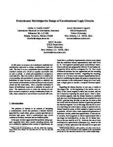
The embedded systems market is without doubt of great economic importance nowadays. The global embedded systems market has doubled in six years passing from US$45 billion in 2003 to roughly US$88 billion in 2009 [1]. For some years now the market has far exceeded that of PC systems. To have an idea of how embedded systems are pervading our daily lives it is sufficient to recall, for example, that there are more than 80 software programs for driving, brakes, petrol control, street finders and air bags installed in the latest car models. As compared with a general-purpose computing system, embedded systems are much more cost sensitive and have strict time-to-market constraints. The design flow of an embedded system features the combined use of heterogeneous techniques, methodologies and tools with which an architectural template is gradually refined step by step on the basis of functional specifications and system requirements. Each phase in the design flow can be seen as a complex optimization problem which is solved by defining and setting some of the system’s free parameters in such a way as to optimize certain performance indexes. These optimization problems are usually tackled by means of processes based on successive cyclic refinements: starting from an initial system configuration, they introduce transformations at each iteration in order to enhance its quality. As in any development process requiring a series of steps towards completion, the presence of cycles is generally a factor which determines its complexity. From a practical viewpoint, a cycle can be schematized as shown in the shaded part in Figure 1. It comprises four basic components: (1) An entry point represented by an initial configuration or set of initial configurations; (2) An evaluation model to measure the validity of a certain configuration; (3) A set of transformations that can be applied to a configuration along with a strategy to apply them (Exploration Strategy); (4) A stop criterion. The definition of efficient optimization strategies based on this type of cycle is often referred to as Design Space Exploration (DSE), a general scheme of which is shown in Figure 1. DSE [2] is addressed differently according to the level of abstraction involved. In this paper we will refer to platform based design [3] with particular reference to ∗ Corresponding Author Email addresses:
[email protected] (Giuseppe Ascia),
[email protected] (Vincenzo Catania),
[email protected] (Alessandro G. Di Nuovo),
[email protected] (Maurizio Palesi),
[email protected] (Davide Patti).
2
Fig. 1. A general design space exploration flow.
the use of parameterized platforms [4]. A parameterized platform is a pre-designed and pre-verified system the components of which can be configured by tuning its parameters. In a parameterized platform for digital camera applications, for example, the parameters could be the configuration of the memory subsystem (e.g. cache memory size, associativity, write policies), application-specific parameters such as the pixel width of a jpeg codec, the size and coding schemes of buses, etc.. The objective of a design space exploration strategy is therefore to determine the optimal value for each parameter in order to optimize certain performance indexes [5–7] (in the previous example, these indexes could be energy consumption and computational performance, e.g. shots per second). Within the DSE flow, the component which mostly affects the weight of an iteration is the evaluation model. The techniques used to evaluate a design depend heavily on the level of abstraction involved [8–11]. The use of mathematical models [12– 14], functional simulators [15–17] and hybrid techniques [18–21] as system-level evaluation tools is particularly suitable during the initial stages of the design flow. In particular, the use of back-annotated functional simulators to evaluate variables that are typically observable at a lower level of abstraction is highly effective as it yields accurate estimates right from the initial design flow phases. With these simulators it is possible to evaluate complex systems which execute entire applications in an acceptable amount of time. Unfortunately their use as evaluation tools in a DSE strategy, which requires evaluation of thousands of system configurations, is confined to small subsystems or simple application kernels. In [22] au3
thors proposed a new methodology that uses a Evolutionary-Fuzzy approach for efficient design space exploration for application specific system-on-a-chip. The Evolutionary-Fuzzy methodology was compared with the state-of-the-art of DSE approaches for embedded computer systems to show that integration of a evolutionary approach with a fuzzy system saves a great amount of time and also gives more accurate results. In this paper we extend our previous work in [22] by proposing a more in-depth description of our Evolutionary-Fuzzy approach and an extensive evaluation of its performance in comparison with state-of-the-art of MOEA methodologies for efficient and accurate exploration of the design space of a parameterized embedded system. The comparison was performed on two systems based on microprocessors belonging to different architectural paradigms. The decision to conduct the analysis using two different case studies was made so as to evaluate how the proposed approach scales as the complexity of the system increases. The rest of the paper is organized as follows. Section 2 outlines some of the main contributions to DSE proposed in the literature. Section 3.1 is a general description of our Evolutionary-Fuzzy approach, which we call MOEA+Fuzzy because it integrates a MOEA with a Fuzzy approximation system. Section 4 presents the simulation framework and the quality measures we used to assess and compare the performances of the proposed algorithm. In Section 5 the methodology is applied to a real case study and evaluated in terms of both efficiency and accuracy, in comparison with state-of-the-art of MOEA methodologies. Finally Section 6 summarizes our contribution and outlines some directions for future work.
2 Related Work
Design space exploration (DSE) is a key issue in embedded system design. In this paper we focus on efficient and accurate DSE of parameterized System on Chip (SoC) platforms. Precisely, we consider a configure-and-excute design paradigm [4] in which, a highly parameterized pre-designed platform is configured, by means of parameter tuning, according to the application (or set of applications) it will have to execute. In this section we first review some of the most relevant contributions in DSE presented in the literature. It will be shown that a common practice consists in minimizing the number of system configurations being visited. However, as the dimension of the design space increases, and the applications to be mapped on the platform become more and more complex, the evaluation of a single system configuration becomes the real DSE bottleneck. A complementary approach is based on minimizing the computational effort needed to evaluate a system configuration. Based on this, a set of relevant contributions aimed at building an approximated model of 4
the system which can be analyzed with a lower effort as compared to the original system, are also reviewed in this section. Finally, we close the section summarizing the main contribution of this work.
2.1 Design Space Exploration Approaches
The main objective of a design space exploration strategy is to minimize the exploration time while guaranteeing good quality solutions. Most of the contributions to the problem of design space exploration to be found in the literature focus on defining strategies for pruning the design space so as to minimize the number of configurations to visit. One exact technique proposed by Givargis et al. in [5] is based on a dependence analysis between parameters. The basic idea is to cluster dependent parameters and then carry out an exhaustive exploration within these clusters. If the size of these clusters increases too much due to great dependency between the parameters, however, the approach becomes a purely exhaustive search, with a consequent loss of efficiency. To deal with these problems several approximate approaches have been proposed which further reduce the exploration space but give no guarantee that the solutions found will be optimal. Fornaciari et al. in [23] use sensitivity analysis to reduce the design space to be explored from the product of the cardinalities of the sets of variation of the parameters to their sum. However, the approach has been presented as a mono-objective approach in which multiple objectives are merged together by means of aggregation functions. Another approximate approach was proposed by Ascia et al. in [6,7], where they proposed a strategy based on evolutionary algorithms for exploration of the configuration space of a parameterized SoC architecture (based on a RISC processor [6] and a VLIW processor [7]) to determine an accurate approximation of the power/performance Pareto-surface. In [24] the authors present an approach to restrict the search to promising regions of the design space. Investigation of the structure of the Pareto-optimal set of design points, for example using a hierarchical composition of sub-component exploration and filtering was addressed in [25,26]. A technique that explicitly models the design space, uses an appropriate abstraction, derives a formal characterization by symbolic techniques and uses pruning techniques is presented in [27].
2.2 Fast Evaluation through Approximated Models
A different approach for reducing the overall exploration time is to minimize the time required to evaluate the system configurations visited. 5
The use of an analytical model to speed up evaluation of a system configuration is presented in [12]. Although the approach is not general (it is fully customized to design space exploration of a memory hierarchy) the authors show that it is possible to compute cache parameters satisfying certain performance criteria without performing simulations or exhaustive exploration. Statistical simulation is used in [28] to enable quick and accurate design decisions in the early stages of computer design, at the processor and system levels. It complements detailed but slower architectural simulations, reducing total design time and cost. A recent approach [29] uses statistical simulation to speed up the evaluation of configurations by a multi-objective evolutionary algorithm. However, the above approaches were developed for and are applicable only to specific cases.
2.3 Coupling Efficient Exploration with Fast System Evaluation
The above discussed techniques can be combined to tackle the DSE problem. That is, an efficient optimization algorithm is used to guide the exploration of the design space, and an approximated model of the system is used to evaluate the system configurations being visited. This approach, known as Multidisciplinary Design Optimization emphasizes the interaction between modeling and optimization. One of the most widespread approaches uses evolutionary algorithms as optimization technique. Broadening the scope to applications not directly connected with the design of an embedded system, the proposals to speedup the evaluation of a single configuration to be found in the literature can be grouped into two main categories: the first comprises methods which use a predefined model that completely replaces the original fitness function [30]; the second category comprises algorithms that evolve the model on-line during the evolution of the evolutionary algorithm, parsimoniously evaluating the original function [31]. The second category can be further subdivided into algorithms that use fixed control during evolution [32,33] and those that use adaptive control [34]. The most popular models for fitness approximation are polynomials (often known as response surface methodology), the Kriging model, whereby Gaussian process models are parameterized by maximum likelihood estimation, most popular in the design and analysis of computer experiments, and artificial neural networks (ANNs). Details of these models are to be found in [35]. In particular in [35], it is stated that ANNs are recommended under the condition that a global model is targeted and that the dimension is high. The reason is that ANNs need a lower number of free parameters compared to polynomials or Gaussian models. Meanwhile, it has been suggested that a combination of local and global models might be necessary. This hypothesis has been confirmed in the following recent work [36]. In the case of multiple objective evolutionary algorithms, a few recent papers have 6
begun to investigate the use of models to approximate fitness evaluations. The study in [37] proposes the use of a neural network approximation combined with the NSGA-II algorithm. Some speedup is observed as compared with using the original exact fitness function alone, but the study is limited to a single, curve-fitting problem. In [38] an inverse neural network is used to map back from a desired point in the objective space (beyond the current Pareto surface) to an estimate of the decision parameters that would achieve it. The test function results presented look particularly promising, though fairly long runs (of 20,000 evaluations) are considered. An algorithm that can give good results with a small number of expensive evaluations is Binary Multiple Single Objective Pareto Sampling (Bin MSOPS) [39,40], which uses a binary search tree to divide up the decision space, and tries to sample from the largest empty regions near fit solutions. Bin MSOPS converges quite quickly and is good in the 1,000–10,000 evaluations range. A recent multi-objective evolutionary algorithm, called ParEGO [41], was devised to obtain an efficient approximation of the Pareto-optimal set with a budget of a few hundred evaluations. The ParEGO algorithm begins with solutions in a latin hypercube and updates a Gaussian process surrogate model of the search landscape after every function evaluation, which it uses to estimate the solution with the largest expected improvement. The effectiveness of these two algorithms is compared in [42].
3 The Multi-Objective Evolutionary Fuzzy (MOEA+Fuzzy) Approach to Speedup Design Space Exploration
3.1 The MOEA+Fuzzy Approach: Motivation and Description
In [6,7] it has been shown how the use of Multi-Objective Evolutionary Algorithms (MOEAs) to tackle the problem of DSE gives optimal solutions in terms of both accuracy and efficiency as compared with the state of the art in exploration algorithms. Unfortunately, EA exploration may still be expensive when a single simulation (i.e., the evaluation of a single system configuration) requires a long compilation and/or execution time. For the sake of example, referring to the computer system architecture considered in this paper, Table 1 reports the computational effort needed for the evaluation (i.e. simulation) of just a single system configuration for several media and digital signal processing application benchmarks. By a little multiplication we can notice that a few thousands of simulations (just a drop in the immense ocean of feasible configurations) could last from a day to weeks! Recently, in [22] authors presented a new methodology that uses a MOEA with 7
Table 1 Evaluation time for a simulation (compilation + execution) for several multimedia benchmarks on a Pentium IV Xeon 2.8 GHz Linux Workstation. Benchmark Description Input size (KB) Simulation time (s) wave
Audio Wavefront computation
625
5.4
g721-enc
CCITT G.711, G.721 and G.723 voice compressions
8
25.9
gsm-dec
European GSM 06.10 full-rate speech transcoding
16
122.4
ieee810
IEEE-1180 reference DCT
inverse
16
37.5
jpeg-codec
jpeg image compression and decompression
32
33.2
mpeg2-enc
MPEG-2 video bitstream encoding
400
245.1
mpeg2-dec
MPEG-2 video bitstream decoding
400
143.7
adpcm-enc
Adaptive Differential Pulse Code Modulation speech encoding
295
22.6
adpcm-dec
Adaptive Differential Pulse Code Modulation speech decoding
16
20.2
fir
FIR filter
64
9.1
fuzzy approximation to speedup the DSE of embedded computer architectures. The Evolutionary-Fuzzy methodology, in comparison with the state-of-the-art of DSE approaches for embedded computers on various multimedia benchmarks, proved to save a great amount of time and also gives more accurate results. In this section we give a more detailed presentation of our Evolutionary-Fuzzy methodology which has the ability to avoid the simulation of configurations that it foresees to be not good enough to belong to the Pareto-set and to give them fitness values according to a fast estimation of the objectives obtained by means of a Fuzzy System (FS). The approach could be informally described as follows: the MOEA evolves normally; in the meanwhile the FS learns from simulations until it becomes expert and reliable. From this moment on the MOEA stops using the simulator as system evaluator and uses the FS to estimate the objectives. Only if the estimated objective values are good enough to enter the Pareto-set will the associated configuration be simulated. It should be pointed out, however, that a “good” configuration might be erroneously discharged due to the approximation 8
Fig. 2. Flow chart of the proposed methodology.
and estimation error. At any rate, this does barely affect the overall quality of the solution found as will be shown in Section 5. Figure 2 describes the evolutionary-fuzzy approach by means of a flow chart. In the training phase the approximator is not reliable and the system configurations are evaluated by means of a simulator which represents the bottleneck of the DSE. The actual results are then used to train the approximator. This cycle repeats until the approximator becomes reliable. From that point on, the system configurations are evaluated by the approximator. If the approximated results are predicted to belong the Pareto set, the simulation is performed. This avoids the insertion in the Pareto set of non-Pareto system configurations. The reliability condition is essential in this flow. It assures that the approximator is reliable and that it can be used in place of the simulator. The reliability test can be performed in several ways as follows: (1) The approximator is considered to be reliable after a given number of samples have been presented. In this case the duration of the training phase is constant and user defined. (2) During the training phase the difference between the actual system output and the predicted (approximated) system output is evaluated. If this difference (error) is below a user defined threshold, the approximator is considered to be reliable. (3) The reliability test is performed using a combination of criteria 1 and 2. That is, during the training phase the difference between the actual system output 9
and the predicted (approximated) system output is evaluated. If this difference (error) is below a user defined threshold and a minimum number of samples have been presented, the approximator is considered to be reliable. The first test is suitable only when the function to approximate is known a priori, so it is possible to preset the number of samples needed by the approximator before the EA exploration starts. In our application the function is obviously not known, so the second test appears to be more suitable. However the design space is wide, for this reason we expect that the error measure oscillates for early evaluations and it will be reliable only when a representative set of system configurations were visited, i.e. a minimum number of configurations were evaluated. So only the third test meets our requirements. The EA and the FS represent the main components of the proposed approach. Whereas the first one is used to generate system configurations to be explored, the second one is used to evaluate them. The next subsections focus on these two important components.
3.2 Genetic Operators and Representation of the Solution Domain
The representation of a system configuration is mapped on a chromosome whose genes define the parameters of the system. The chromosome has as many genes as the number of free parameters and each gene is coded according to the set of values the parameter can take. For instance Figure 3 shows our reference parameterized architectures, which will be presented in Section 4, and its mapping on the chromosome. For each objective to be optimized it is necessary to define the respective measurement functions. These functions, which we will call objective functions, frequently represent cost functions to be minimized. (e.g. area, power, delay, etc.). Crossover (recombination) and mutation operators produce the offspring. In our specific case, the mutation operator randomly modifies the value of a parameter
Fig. 3. From system to chromosome.
10
chosen at random. The crossover between two configurations exchanges the value of two parameters chosen at random. Application of these operators may generate non-valid configurations (i.e. ones that cannot be mapped on the system). Although it is possible to define the operators in such a way that they will always give feasible configurations, or to define recovery functions, these have not been taken into consideration in the paper. Any unfeasible configurations are filtered by the feasible function. A feasible function fF : C −→ {true, f alse} assigns a generic configuration c belonging to the configuration space C a value of true if it is feasible and f alse if c cannot be mapped onto the parameterized system. A fixed number of either fitness evaluations or generations is used as stop criteria.
3.3 Fuzzy Function Approximation
The MOEA+Fuzzy approach uses a k-level Hierarchical Fuzzy System (HFS), which has been demonstrated to be a universal approximator [43]. The HFS is generated as a cascade of single fuzzy sub-systems. Each fuzzy sub-system is used to model a particular component of the embedded system. In this hierarchical fuzzy system the outputs of the fuzzy sub-system at level l − 1 are used as inputs to the fuzzy sub-system at level l. This hierarchical decomposition of the system allows us to reduce drastically the complexity of the estimation problem with the additional effect of improving estimation accuracy. Single fuzzy systems are generated with a method that is based on the well-known Wang and Mendel method [44], which consists of five steps: • Step 1 Divides the input and output space of the given numerical data into fuzzy regions; • Step 2 Generates fuzzy rules from the given data; • Step 3 Assigns a degree to each of the generated rules for the purpose of resolving conflicts among them (rule with higher degree wins); • Step 4 Creates a combined fuzzy rule base based on both the generated rules and, if there were any, linguistic rules previously provided by human experts; • Step 5 Determines a mapping from the input space to the output space based on the combined fuzzy rule base using a defuzzifying procedure. From Step 1 to 5 it is evident that this method is simple and straightforward, in the sense that it is a one-pass buildup procedure that does not require time-consuming training. In our implementation the output space could not be divided in Step 1, because we had no information about boundaries. For this reason we used Takagi-Sugeno fuzzy rules [45], in which each i-th rule has as consequents M real numbers siz , with z ∈ [1, M], associated with all the M outputs. 11
Fig. 4. Fuzzy Rule Generation Example.
T Sj being the set of fuzzy sets associated with the variable xj , the fuzzy rules Ri of the single fuzzy subsystem are defined as: Ri : if x1 is Si1 and . . . and xN is SiN then yi1 = si1 , . . . , yim = siM where Sij ∈ T Sj . Let αjk be the degree of truth of the fuzzy set Sjk belonging to T Sj corresponding to the input value x¯j . If mj is the index such that αjmj is the greatest of the αjk , the rule Ri will contain the antecedent xj is Sjmj . After constructing the set of antecedents the consequent values yiz equal to the values of the outputs are associated. The rule Ri is then assigned a degree equal to the product of the N highest degrees of truth associated with the fuzzy sets chosen Sij . Let us assume that we are given a set of two input - one output data pairs: (x1 , x2 ; y), and a total of four fuzzy sets (respectively LOW1 , HIGH1 and LOW2 , HIGH2 ) associated with the two inputs. Let us also assume that x1 has a degree of 0.8 in HIGH1 and 0.2 in LOW1 , and x2 has a degree of 0.4 in HIGH2 and 0.6 in LOW2 , y = 10. As can be seen from Figure 4, the fuzzy sets with the highest degree of truth are LOW1 and HIGH2 , so the rule generated would be: if x1 is HIGH1 and x2 is LOW2 then y = 10. The rule degree is 0.8×0.6 = 0.48. The rules generated in this way are ”and” rules, i.e., rules in which the condition of the IF part must be met simultaneously in order for the result of the THEN part to occur. For the problem considered in this paper, i.e., generating fuzzy rules from numerical data, only ”and” rules are required since the antecedents are different components of a single input vector. Steps 2 to 4 are iterated with the EA: after every evaluation a fuzzy rule is created and inserted into the rule base, according to its degree in case of conflicts. More specifically, if the rule base already contains a rule with the same antecedents, the degrees associated with the existing rule are compared with that of the new rule and 12
the one with the highest degree wins. For example consider another input/output vector where x1 has a degree of 0.9 in LOW1 and 0.7 in HIGH2 , y = 8. As can be seen from Figure 4, the fuzzy sets with the highest degree of truth are LOW1 and HIGH2 , so the rule generated would have the same antecedents of the previous rule but different consequent. The rule with the highest degree wins (in our example it is the second rule with a degree of 0.63 against 0.48). In Step 5 the defuzzifying procedure to calculate the approximated output value yˆ is the one suggested in [44]. According to this method the defuzzified output is determined as follows
yˆj =
K P
mr y¯rz
r=1 K P
r=1
(1) mr
where K is the number of rules in the fuzzy rule base, y¯rz is the output estimated by the r-th rule for the z-th output and mr is the degree of truth of the r-th rule. In our implementation the defuzzifying procedure and the shape of the fuzzy sets were chosen a priori. This choice proved to be effective as well as a more intelligent implementation which could embed a selection procedure to choose the best defuzzifying function and shape to use online. The advantage of our implementation is a lesser complexity of the algorithm and a faster convergence without appreciable losses in accuracy as will be shown in the rest of the paper. Additional details on the hierarchical system used in our tests are in Section 4.2.
4 Simulation Framework and Quality Measures
In this section we present the simulation framework we used to evaluate the objectives to be optimized, and the quality measures we used to assess different approaches. 4.1 Parameterized System Architecture and Simulation Flow
Architectures based on Very Long Instruction Word (VLIW) processors [46] are emerging in the domain of modern, increasingly complex embedded multimedia applications, given their capacity to exploit high levels of performance while maintaining a reasonable trade-off between hardware complexity, cost and power consumption. A VLIW architecture, like a superscalar architecture, allows several in13
Fig. 5. Simulation flow.
structions to be issued in a single clock cycle, with the aim of obtaining a good degree of Instruction Level Parallelism (ILP). To evaluate and compare the performance indexes of different architectures for a specific application, one needs to simulate the architecture running the code of the application. When the architecture is based on a VLIW processor this is impossible without a compiler because it has to schedule instructions. In addition, to make architectural exploration possible both the compiler and the simulator have to be retargetable. Trimaran [16] provides these tools and thus represents the pillar central to the EPIC-Explorer [20], which is a framework that not only allows us to evaluate any instance of a platform in terms of performance (i.e. the execution time) and power dissipated, exploiting the state of the art in estimation approaches at a high level of abstraction, but also implements various techniques for exploration of the design space. The EPIC-Explorer platform, which can be freely downloaded from the Internet [47], allows the designer to evaluate any application written in C and compiled for any instance of the platform. For this reason it is an excellent testbed for comparison between different design space exploration algorithms. The tunable parameters of the architecture can be classified in three main categories: • Register files. Each register file is parameterized with respect to the number of registers it contains. These include a set of general purpose registers (GPR) comprising 32-bit registers for integers with or without sign; FPR registers comprising 64-bit registers for floating point values (with single and double precision); Predicate registers (PR) comprising 1-bit registers used to store the Boolean values of instructions using predication; and BTR registers comprising 64-bit registers containing information about possible future branches. • The functional units. Four different types of functional units are available: integer, floating point, memory and branch. Here parametrization regards the number of instances for each unit. • The memory sub-system. Each of the three caches, level 1 data cache, level 1 instruction cache, and level 2 unified cache, is independently specified with the following parameters: size, block size and associativity. Each of these parameters can be assigned a value from a finite set of values. A 14
complete assignment of values to all the parameters is a configuration. A complete collection of all possible configurations is the configuration space, (also known as the design space). A configuration of the system generates an instance that is simulated and evaluated for a specific application according to the scheme in Figure 5. The application written in C is first compiled. Trimaran uses the IMPACT compiler system as its front-end. This front-end performs ANSI C parsing, code profiling, classical code optimizations and block formation. The code produced, together with the High Level Machine Description Facility (HMDES) machine specification, represents the Elcor input. The HMDES is the machine description language used in Trimaran. This language describes a processor architecture from the compiler’s point of view. Elcor is Trimaran’s back-end for the HPL-PD architecture and is parameterized by the machine description facility to a large extent. It performs three tasks: code selection and scheduling, register allocation, and machine dependent code optimizations. The Trimaran framework also consists of a simulator which is used to generate various statistics such as compute cycles, total number of operations, etc. In order to consider the impact of the memory hierarchy, a cache simulator has been added to the platform. Together with the configuration of the system, the statistics produced by simulation contain all the information needed to apply the performance and power consumption estimation models. The results obtained by these models are the input for the exploration block. This block implements an optimization algorithm, the aim of which is to modify the parameters of the configuration so as to minimize the two cost functions (execution time and power dissipation). The performance statistics produced by the simulator are expressed in clock cycles. To evaluate the execution time it is sufficient to multiply the number of clock cycles by the clock period. This was set to 200MHz, which is long enough to access cache memory in a single clock cycle.
4.2 The Hierarchical Fuzzy System
The estimation block of the framework consists of a Hierarchy of Fuzzy Systems that models the embedded system shown in Figure 6. This system is formed by three levels: the processor level, the L1 cache memory level, and the L2 cache memory level. A FS at level l uses as inputs the outputs of the FS at level l − 1. For example, the FS used to estimate misses and hits in the first-level instruction cache uses as inputs the number of integer operations, float operations and branch operations estimated by the processor level FS as well as the cache configuration (size, block size, and associativity). The knowledge base was defined on the basis of experience gained from an extensive series of tests. Our aim was to obtain the maximum approximation accuracy. 15
Fig. 6. A block scheme of the Embedded System used. SoC components (Proc, L1D$,L1I$ and L2D$) are modeled with a MIMO Fuzzy System, which is connected with others following the SoC hierarchy.
We therefore chose to use the maximum granularity in all our experiments; in fact we chose to describe each input variable with as many membership functions (i.e. the number of fuzzy sets in the term set) as the number of values available for that input variable. It is not possible to know the range of variation of subset input variables that are also output variables of the previous level (chained variables). It is thus not possible to use the same approach as for the other variables. We therefore fixed a constant number of fuzzy sets that are rescaled on-line during the DSE according to variations in the range for the variable(s) they are associated with. Following a number of tests we chose to use 9 fuzzy sets for these chained variables. As the maximum number of rules in a fuzzy system is
N Q
Cj , where Cj is the cardinal-
j=1
ity of the term set T Sj for the variable xj , the fuzzy system could potentially have thousands of rules. This is not a problem: we verified, in fact, that a fuzzy system with a few thousand rules takes milliseconds to approximate the objectives, which is some orders of magnitude less than the time required for simulation. The shape chosen for the sets was always an equidistant Gaussian intersecting each other at a degree of 0.5. As an example, Figure 7 shows the term sets for a 2-level hierarchical fuzzy system which approximates a memory hierarchy with 2 cache levels. At level 1 there are 2 fuzzy subsystems modeling the data cache (FS L1D$) and the instruction cache (FS L1I$); at level 2 there is the fuzzy system FS L2U$ whose inputs include two chained variables: the number of misses of the two caches of the previous level. The fuzzy sets associated with each input are equidistant with a Gaussian shape.
4.3 Assessment of Pareto set Approximation
It is difficult to define appropriate quality measures for Pareto set approximations, and as a consequence graphical plots were until recently used to compare the out16
Fig. 7. Example of an HFS, which models the 2 level memory hierarchy.
comes of MOEAs. Nevertheless quality measures are necessary in order to compare the outcomes of multi-objective optimizers in a quantitative manner. Several quality measures have been proposed in the literature in recent years, an analysis and review of these is to be found in [48]. In this work we follow the guidelines suggested in [49], which is a recent tutorial on performance assessment of stochastic Multi-Objective Optimizers. The quality measures we considered most suitable for our context are the followings: (1) Hypervolume, This is a widely-used index, which measures the hypervolume of that portion of the objective space that is weakly dominated by the Pareto set to be evaluated. In order to measure this index the objective space must be bounded- if it is not, then a bounding reference point that is (at least weakly) dominated by all points should be used. In this work we define as bounding point the one which has coordinates in the objective space equal to the highest values obtained. Higher quality corresponds to smaller values. (2) Pareto Dominance, the value this index takes is equal to the ratio between the total number of points in Pareto set P that are also present in a reference Pareto set R (i.e. it is the number of non-dominated points by the other Pareto set). In this case a higher value obviously corresponds to a better Pareto set. Using the same reference Pareto set, it is possible to compare quantitatively results from different algorithms. (3) Distance, this index explains how close a Pareto set (P ) is to a reference set (R). We define the average and maximum distance index as follows: distanceavg =
X x∈P
min(d(x, y)), y∈R
distancemax = max(min(d(x, y))), x∈P
17
y∈R
where x and y are vectors whose size is equal to the number of objectives, M, and d(·, ·) is the Euclidean distance. The lower the value of this index, the more similar the two Pareto sets are. For example a high value of maximum distance suggest that some reference points are not well approximated, and consequently a high value of average distance tells us that an entire region of the reference Pareto is missing in the approximated set. A standard, linear normalization procedure was applied to allow the different objectives to contribute approximately equally to index values. When the Pareto-optimal set is not available, we could only compare the relative quality of Pareto-sets achieved by various algorithms. So we used the following approach to obtain a reference Pareto-set: first, we combined all approximations sets generated by the algorithms under consideration, and then the dominated objective vectors are removed from this union. At last, the remaining points, which are not dominated by any of the approximations sets, form the reference set. The advantage of this approach is that the reference set weakly dominates all approximation sets under consideration. For the analysis of multiple runs, we compute the quality measures of each individual run, and report the mean and the standard deviation of these. Since the distribution of the algorithms we compare are not necessarily normal, we use a nonparametric test to indicate if there is a statistically significant difference between distributions: the Mann-Whitney rank-sum test to compare two distributions. We recall that the significance level of a test is the maximum probability, assuming the null hypothesis, which the statistic will be observed, i.e. the null hypothesis will be rejected in error when it is true. The lower the significance level, the stronger the evidence.
5 Experiments and Results
In this section we will evaluate the approach presented in section 3.1 on two systems based on a Very Long Instruction Word (VLIW) microprocessor. The first one is based on a commercially available VLIW microprocessor core from STMicroelectronics, the LX/ST200 [50], targeted for multimedia applications. The second one is a completely customizable (parameterized) VLIW architecture. The decision to conduct the analysis using two different case studies was made so as to evaluate how the proposed approach scales as the complexity of the system increases. As will be described in the following subsections, the design space of the LX/ST200 system is much smaller than that of the completely customizable VLIW. The limited size of the design space in the first case will thus allow us to evaluate the approach and compare it with an exhaustive exploration. 18
In this research we compare our approach with SPEA2 (MOEA), NSGA-II with ANN approximation (NSGA2+ANN), ParEGO and Bin MSOPS. The ParEGO and Bin MSOPS algorithms were provided from the authors and we used the default settings, as described in [42]. Parameters of the MOEA, MOEA+Fuzzy and NSGA2+ANN are as follows: The internal and external population for the evolutionary algorithm were set as comprising 30 individuals, using a crossover probability of 0.8 and a mutation probability of 0.1. These values were set in order to maximize the performance over the short run experiments, following the indications given in [6], where the convergence times and accuracy of the results were evaluated with various crossover and mutation probabilities, and it was observed that the performance of the algorithm with the various benchmarks was very similar. That is, the optimal GA parameters seem to depend much more on the architecture of the system than on the application. This makes it reasonable to assume that the GA parameter tuning phase only needs to be performed once (possibly on a significant set of applications). The GA parameters thus obtained can then be used to explore the same platform for different applications. The approximation error in MOEA+Fuzzy is calculated in a window of 20 simulations for the objectives, and the reliability threshold was set to 5% of the Euclidean distance between the real point (individuated by the simulation results) and the approximate one in the objective space. The minimum simulations threshold was set to 90. Both thresholds were chosen after extensive series of experiments with computationally inexpensive test functions. The NSGA2+ANN approach was directly derived from our MOEA+Fuzzy by using ANNs instead of FSs to model the embedded system components. In this case NSGA-II was chosen as MOEA because in our preliminary tests NSGA-II works slightly better than SPEA-2 in conjunction with ANN, therefore we found in the literature only works that integrate NSGA-II with ANN [38,35], but no work that integrates SPEA-2 with ANN is present. Every ANN structure is obtained following the hints in [51]. The ANN structure is a Multi-Layer Perceptron (MLP) obtained by an off-line optimization phase, where 100 random system configurations were simulated and used to design the suitable ANN structure for the specific DSE problem being addressed. These 100 simulations were included in the total number of simulations done by the NSGA2+ANN. Only the weights were adapted on-line in every single DSE, using the Resilient backpropagation (RPROP) algorithm [52]. The implementation of NSGA-II that we use is the one available for download from Deb’s KANGAL web page [53]. We use default settings, as supplied, with one exception the population size is reduced to 30. We remark that in both tests the resulting Pareto solutions have a finite number of elements due to the limited set of integer parameters. The discontinuities of the Pareto front results from the discontinuities in the parameters space. Such limitations are mainly due to the actual architectural and micro-architectural constraints on the modules which form the datapath of the system architecture. For the sake of example, cache size does not varies linearly from minimum to maximum cache 19
Table 2 Design space for the LX/ST200 based system. Parameter
Parameter space
L1D cache size
2KB,4KB...,128KB
L1D cache block size L1D cache associativity L1I cache size
16B,32B,64B 1,2 2KB,4KB...,128KB
L1I cache block size
16B,32B,64B
L1I cache associativity L2U cache size
1,2 128KB,...,512KB
L2U cache block size L2U cache associativity Space size
32B,64B,128B 2,4,8 47, 628
size but it varies by powers of two. In the rest of the paper we indicate with the term number of simulations the actual number of times a simulation is run, whereas, with number of generations, we refer to the number of iterations of the evolutionary process which involves the selection, the reproduction and the fitness evaluation. Please note that this latter could result in either a system-level simulation or a system-level evaluation carried out by means of a Fuzzy System or a Neural Network. Finally, the number of runs is the number of times the algorithms are repeated.
5.1 A Case Study: Application Specific Cache Customization
To evaluate the accuracy of the approach we considered the problem of exploring the design space of a system comprising the STMicroelectronics LX/ST200 VLIW processor and a parameterized 2-level memory hierarchy. This choice was made because the size of the design space and the time required to evaluate a configuration for this architecture are sufficiently small as to make an exhaustive exploration computationally feasible. The 2-level memory hierarchy consists of a separated first level instruction and data cache and a unified second-level cache. The parameter space along with the size of the design space to be explored is reported in Table 2. Table 3 summarizes the exploration results for gsm-decode application. The evaluation of a single system configuration running gsm-decoding application requires about 2 minutes to be executed by an instrumented LX/ST200 instruction 20
Table 3 Exhaustive, MOEA, MOEA+Fuzzy, NSGA2+ANN and Bin MSOPS explorations comparisons for GSM-decode application Approach
Simulations
Total time
Pareto-optimal
required
points discovered
(average)
(%)
Hypervolume
Average Distance
Max Distance
(%)
(%)
Exhaustive
43416
2 months
100.00%
52.61
0.0000
0.0000
MOEA
5219.2
1 week
100.00%
52.61
0.0000
0.0000
MOEA+Fuzzy
749.5
1 day
90.76%
52.60
0.0098
0.1895
NSGA2+ANN
682.3
1 day
88.80%
52.59
0.0102
0.2015
Bin MSOPS
8614.2
1.5 weeks
12.31%
48.21
0.4297
2.4539
set simulator 1 on a Pentium IV Xeon 2.8GHz workstation. The following exploration strategies were compared: exhaustive exploration in which each feasible configuration of the design space was evaluated, the approach proposed in [6] which uses SPEA2 as the optimization algorithm (MOEA), the approach proposed in this paper, which uses SPEA2 as the optimization algorithm and fuzzy systems as approximation models (MOEA+Fuzzy), the NSGA-II with ANN modeling (NSGA2+ANN) and the Bin MSOPS. For each approach the Table 3 reports the total number of configurations simulated and the values of the performance indexes discussed in Section 4. For the approaches using EAs, the reported values are averaged over 100 runs. As can be observed in Table 3, the number of configurations simulated during exhaustive exploration is lower than the size of the design space. This is due to the fact that some of the configurations (about 10%) are unfeasible. ParEGO results are not present, because it is not suitable with numbers of iterations larger than very few hundreds [41]. In fact ParEGO convergence becomes progressively slower as number of configurations visited increases. For this reason its results do not improve significantly after a few generations. In this case study the Pareto-optimal set is available, so it is the reference set for all comparisons reported in this subsection. The results are represented in tables using the mean and standard deviation (the latter in brackets) of the performance indexes. With the MOEA approach all points of the Pareto-optimal set are obtained after about 250 generations, visiting on average slightly over 5,000 configurations. From Table 3 it can be seen that the MOEA+Fuzzy approach, which converges after about 250 generations like the MOEA approach, offers a great saving in the time required for exploration at the average cost of 10% of the Pareto-optimal points. Considering 1
The LX/ST200 instruction-set simulator has been instrumented with an instruction-level power model which allows to estimate the average power dissipation with an accuracy of 5% as compared with a gate level power analysis [54].
21
Table 4 Random search, SPEA2 (MOEA), NSGA-II+ANN (NSGA2+ANN), MOEA+Fuzzy, ParEGO and Bin MSOPS comparisons on a budget of 250 simulations. Approach
Hypervolume
Distance (%)
Pareto Dominance
(%)
average
maximum
(%)
Random search
29.30 (1.44)
4.25 (0.30)
9.93 (0.75)
0.33 (0.11)
MOEA
50.54 (0.32)
0.21 (0.08)
0.83 (0.53)
13.85 (4.43)
MOEA+Fuzzy
52.30 (0.09)
0.06 (0.02)
0.41 (0.22)
46.15 (1.45)
NSGA2+ANN
52.32 (0.44)
0.08 (0.07)
0.88 (0.41)
34.92 (5.28)
ParEGO
35.60 (0.37)
3.14 (0.09)
7.66 (0.57)
0.51 (0.23)
Bin MSOPS
34.55 (1.12)
4.30 (0.29)
14.05 (2.16)
0.77 (0.42)
In this case Pareto Dominance index assesses the Pareto-optimal points discovered.
hypervolume and distance, we see that the Pareto set obtained by the MOEA+Fuzzy approach is highly representative of the complete set, so the missing points can be considered negligible. Similar results were obtained with NSGA2+ANN, which in this test could be considered as good as MOEA+Fuzzy. In contrast Bin MSOPS results come close to a random search, as is confirmed in Table 4. This is due to the low accuracy of its model. Table 4 gives the results (hypervolume and distance between approximated Paretos and the Pareto-optimal set) obtained on a budget of 250 simulations by a random search, MOEA, MOEA+Fuzzy, NSGA2+ANN and the ParEGO and Bin MSOPS algorithms. The Pareto-set obtained by MOEA+Fuzzy after just 250 simulations is very close to the Pareto-optimal set (average distance is 0.06 %) and little less than 50% of the Pareto-optimal points were already discovered. All the indexes calculated in the experiment with 250 simulations confirm a significant improvement in quality by MOEA when the fuzzy approximation system is used. Once again the NSGA2+ANN average results are as good as those obtained by MOEA+Fuzzy, while the standard deviation is higher because the final result depends greatly on the configurations simulated in the early generations, which are chosen practically at random. As expected, the results obtained by ParEGO and Bin MSOPS confirm that both the algorithms are not suitable to tackle DSE problems. The main reason for the low quality of the solutions found is mainly related to the high dimensionality, the integer nature of the input parameter space, and the roughness and sharpness of the fitness landscape which characterizes such systems. This is also confirmed by the Kruskal-Wallis test where the results found by Bin MSOPS algorithm are not so significant as compared to pseudo-random search (it is clearly visible in Figure 8(a) that reports box plots for hypervolume distributions). This is mostly 22
50
0.66 MOGA+Fuzzy MOGA
0.64
40
0.62
0.6
35
Hypervolume
Hypervolume (%)
45
30
0.58
0.56
0.54
0.52
0.5
25 0.48
MOGA
MOGA+ANNMOGA+FUZZY
ParEGO
BIN_MSOPS
RANDOM
0.46
0
100
200
300
400
500
600
700
800
Number of Simulations
(a)
(b)
Fig. 8. Box plot for hypervolume (a). Hypervolume evolution (b).
Fig. 9. Results of all configurations simulated with Exhaustive (light grey), MOEA (dark grey), MOEA+Fuzzy (black) approaches. Each configuration simulated gives a pair of objective values (i.e. results), which are the coordinates of the points in this Figure.
due to the roughness of the functions to approximate, which are nonlinear. Figure 8(b) shows the trend of the hypervolume for MOEA and MOEA+Fuzzy as the number of simulations increases. As can be seen, the MOEA and MOEA+Fuzzy approaches proceed equally until the approximator becomes reliable. At this point MOEA+Fuzzy decidedly speeds up after a few generations, which are equivalent to a few tens of simulations, and converges after a few hundred simulations. MOEA is slower to converge: only after about a thousand simulations it is able to produce a better Pareto set than the one found by MOEA+Fuzzy. Figure 9 shows the objective space for all configurations simulated by exhaustive exploration (light grey), by MOEA (dark grey) and by MOEA+Fuzzy (black). Each configuration simulated gives a pair of objective values (i.e. results), which are used as coordinates for the points depicted in Figure 9. As can be seen, the configurations explored by the MOEA+Fuzzy approach are distributed with greater 23
Table 5 Design space of the parameterized VLIW based system architecture. Parameter
Parameter space
Integer Units
1,2,3,4,5,6
Float Units
1,2,3,4,5,6
Memory Units
1,2,3,4
Branch Units
1,2,3,4
GPR/FPR
16,32,64,128
PR/CR
32,64,128
BTR
8,12,16
L1D/I cache size
1KB,2KB,...,128KB
L1D/I cache block size
32B,64B,128B
L1D/I cache associativity L2U cache size
1,2,4 32KB,64KB...,512KB
L2U cache block size
64B,128B,256B
L2U cache associativity
2,4,8,16 7.739 × 10¹⁰
Space size
density around the Pareto optimal set. Numerically this concept is explained by the average distance of all points from the Pareto optimal set, that is 3.72% for MOEA+Fuzzy (the maximum distance is 52.41%) against 5.31% (the maximum distance is 64.16%) of MOEA. This confirms that the MOEA+Fuzzy is capable to identify less promising configurations and it avoids to waste time to simulate them.
5.2 Design Space Exploration of a Parameterized VLIW-based Embedded System
In this subsection we present a comparison between the performance of MOEA, ParEGO and our MOEA+Fuzzy approach. Bin MSOPS was not considered because it does not work well with larger decision spaces. In this study we repeated the execution of the algorithms 10 times using different random seeds. The eighteen input parameters, along with the size of the design space for the parameterized VLIW based system architecture being studied, are given in Table 5. As can be seen from Table 5, the size of the configuration space is such as to be able to explore all the configurations in a 365-day year a simulation needs to last about 3 ms, a value which is several orders of magnitude away from the values in Table 1. A whole human lifetime would not, in fact, be long enough to obtain 24
complete results for an exhaustive exploration of any of the existing benchmarks, even using the most powerful workstation currently available. Even if we use High Performance Computing systems, they will be extremely expensive (in terms of money) and will still require a long time. Essentially DSE must identify some suitable configurations, among the enormous space in Table 5, for in-depth studies at lower design levels. DSE is a crucial highlevel design procedure, so even a less efficient decision in this phase could doom the entire design process to failure. However, a well-known market law says that the first product to appear wins over late-comers and, more interestingly, it can be sold at the highest price. So it is preferable for DSE not to be time-consuming. For this reason it is not necessary to discover all the Pareto-optimal configurations, but only some of them and/or some very good quality approximations. Keeping this in mind, we decided to carry out two different tests to compare the performance of our approach with that of others. The first test was performed on a budget of 250 simulations, because we consider it to be a good milestone in DSE. Even in the case of the most time-consuming benchmark, in fact, 250 simulations take about 8 hours (i.e. it is possible to leave a workstation to explore overnight and to have the results the next morning). In the second test we compared the Pareto sets obtained after 100 generations, with an unconstrained number of simulations, to assess performance and quality when longer runs are possible. The decision to limit the number of generations to 100 was due to the fact that after this threshold hardly any significant difference is observed in the quality of the Pareto sets obtained, i.e. after this threshold no significant improvement that would justify further simulations is expected. The results are represented in tables using the mean and standard deviation (the latter in brackets) of the performance indexes obtained from the compared algorithms (columns) in the nine benchmarks (rows). In the first test on 250 simulations we focused only on quality of results, and the research proved that the proposed MOEA+Fuzzy approach outperforms the competitors in terms of both hypervolume and Pareto dominance indexes. In fact MOEA+Fuzzy comes out on top in seven out of nine benchmarks in the Pareto dominance index comparison, as shown in Table 6. The NSGA2+ANN is significantly better than MOEA only in three cases out of nine. The hypervolume comparison, Table 7 in which algorithms that use approximation techniques are compared with the standard MOEA, shows that MOEA+Fuzzy is significantly better than MOEA in five out of nine test cases, and it obtains the best result in six cases. Meanwhile NSGA2+ANN is significantly better in two out of nine test cases, and it obtains the best results in three cases. Considering the two indexes, we can see that MOEA+Fuzzy always discovers a good number of highquality points over the Pareto front, which is the most important feature in DSE. Graphic confirmation of the quality of the results obtained by MOEA+Fuzzy is to 25
Table 6 Pareto Dominance, a comparison between ParEGO, SPEA2 (MOEA), NSGA-II+ANN (NSGA2+ANN) and MOEA+Fuzzy on a budget of 250 simulations. Benchmark
Pareto Dominance (%)
Mann-Withney test
mean (standard deviation)
significance level
MOEA
MOEA+Fuzzy
NSGA2+ANN
ParEGO
α at 1%
wave
15.80 (9.09)
65.99 (13.17)
17.29 (8.42)
0.92 (1.69)
MOEA+Fuzzy wins
fir
14.49 (9.00)
47.42 (14.28)
35.05 (13.30)
3.05 (3.70)
adpcm-encode
9.74 (6.99)
61.30 (17.07)
27.35 (17.46)
1.61 (1.72)
MOEA+Fuzzy wins
adpcm-decode
9.11 (6.18)
64.98 (14.61)
25.92 (17.18)
0.00 (0.00)
MOEA+Fuzzy wins
g721-encode
22.10 (12.40)
39.76 (18.50)
25.99 (21.37)
12.14 (7.61)
none
ieee810
16.17 (3.70)
63.92 (4.34)
19.91 (5.86)
0.00 (0.00)
MOEA+Fuzzy wins
jpeg-codec
17.21 (14.55)
32.99 (23.64)
46.77 (29.01)
3.03 (6.45)
MOEA+Fuzzy & NSGA2+ANN
mpeg2-encode
19.29 (10.26)
40.82 (13.78)
32.00 (18.45)
7.87 (5.10)
MOEA+Fuzzy & NSGA2+ANN
mpeg2-decode
26.03 (11.40)
21.42 (5.78)
42.67 (16.53)
9.88 (5.98)
MOEA+Fuzzy & NSGA2+ANN
In this case, unlike the others, in building the reference Pareto sets we considered the sets obtained by all the approaches after 250 simulations. Algorithms that use approximation techniques are compared with the standard MOEA. An algorithm “wins” when its results are better than MOEA with statistical significance level α at 1%.
be found in Figures 10 and 11, which show the best Pareto set obtained by each algorithm by means of the union of the best points from the Pareto sets it obtained in the various executions. According to the results shown in Tables 6 and 7, the MOEA+Fuzzy demonstrated that it significantly improves the results obtained by the standard MOEA approach. NSGA2+ANN also demonstrated that it could improve the standard MOEA approach, but its results are significantly better only in two cases out of nine. In Tables 6 and 7 it can also be observed that NSGA2+ANN obtains significantly better results than MOEA only when MOEA+Fuzzy does the same.
26
none
Table 7 Hypervolume, a comparison between ParEGO, SPEA2 (MOEA), NSGA-II+ANN (NSGA2+ANN) and MOEA+Fuzzy on a budget of 250 simulations Benchmark
Hypervolume (%)
Best algorithm according to
mean (standard deviation)
Mann-Withney test
MOEA
MOEA+Fuzzy
NSGA2+ANN
ParEGO
significance level α at 1%
wave
53.72 (2.93)
67.87 (1.59)
57.73 (3.25)
37.21 (8.36)
MOEA+Fuzzy wins
fir
57.88 (3.89)
61.19 (1.51)
60.42 (1.72)
51.25 (8.45)
none
adpcm-encode
62.66 (2.63)
66.66 (1.45)
66.02 (2.71)
55.49 (3.24)
MOEA+Fuzzy wins
adpcm-decode
20.95 (5.64)
40.96 (3.21)
38.13 (9.18)
9.12 (1.66)
g721-encode
78.88 (1.23)
79.46 (1.36)
79.53 (1.76)
75.28 (0.15)
ieee810
65.90 (0.98)
75.19 (0.55)
74.79 (0.76)
58.27 (4.11)
jpeg-codec
72.90 (2.82)
73.95 (4.12)
76.18 (6.39)
55.71 (22.00)
none
mpeg2-encode
66.81 (2.98)
70.86 (1.25)
69.33 (3.11)
56.16 (5.70)
MOEA+Fuzzy wins
mpeg2-decode
84.18 (0.41)
84.76 (1.32)
85.76 (1.89)
83.88 (0.64)
none
MOEA+Fuzzy & NSGA2+ANN none MOEA+Fuzzy & NSGA2+ANN
Algorithms that use approximation techniques are compared with the standard MOEA. An algorithm “wins” when its results are better than MOEA with statistical significance level α at 1%.
27
0.13 MOEA+Fuzzy MOEA MOEA+ANN ParEGO
0.125
Execution Time (ms)
0.12 0.115 0.11 0.105 0.1 0.095 0.09 0.085 1.5
1.6
1.7
1.8 1.9 2 2.1 2.2 Average Power Consumption (W)
2.3
2.4
2.5
Fig. 10. wave: Best Pareto sets and attainment surfaces obtained by MOEA, MOEA+Fuzzy, NSGA2+ANN and ParEGO on a budget of 250 simulations.
28
MOEA MOEA+Fuzzy MOEA+ANN ParEGO
60
Execution Time (ms)
55
50
45
40 1.4
1.5 1.6 1.7 1.8 Average Power Consumption (W)
1.9
Fig. 11. adpcm-decode: Best Pareto sets and attainment surfaces obtained by MOEA, MOEA+Fuzzy, NSGA2+ANN and ParEGO on a budget of 250 simulations.
29
In the second test, time requirements were also taken into account, and results were assessed as a trade-off between performance and the length of time required. From Table 9, which gives the hypervolume, and Table 10, which gives the Pareto distance obtained by MOEA, MOEA+Fuzzy and NSGA2+ANN after 100 generations, it can be observed that only MOEA+Fuzzy yields a similar result to that of the approach based on MOEA. The consideration that the Pareto sets obtained by MOEA and MOEA+Fuzzy are practically equal, as can be seen graphically from two representative examples in Figures 14 and 15, is numerically justified by the short distance between the two sets and the statistical equality between the hypervolumes. In fact we can observe that the hypervolume indexes are very close in all the benchmarks and that the average distance between the reference Pareto sets and the MOEA+Fuzzy Pareto sets is 1.2034%, an excellent result compared with the 0.8288% obtained by MOEA and the 2.1078% obtained by NSGA2+ANN. In fact we can state that the MOEA+Fuzzy results are practically equal to the MOEA ones, and they are better than NSGA2+ANN. Therefore the MOEA+Fuzzy results are not statistically different from the MOEA ones, whereas the NSGA2+ANN results are statistically different. Although the NSGA2+ANN results are on average similar to those obtained by MOEA+Fuzzy they have a greater variance and so in most cases it is not statistically possible to state that executing NSGA2+ANN gives a reasonable certainty of results that are better or comparable with those of the standard MOEA. This is because the performance of NSGA2+ANN is affected by the choice of the first configurations simulated, which are the basis for the learning phase. They are chosen practically at random given that in the early generations the GA has not yet started to converge. As regards the efficiency of the proposed approach, Table 8 gives the number of system configurations simulated by MOEA, MOEA+Fuzzy and NSGA2+ANN. Comparisons exhibit an average 66% saving on exploration time, which may mean several hours or almost a day depending on the benchmark (from about 3 hours for wave to 5 days for mpeg2-encode). NSGA2+ANN executes fewer simulations, saving 71% of the time needed, but, as shown in Tables 9 and 10, this comes at the cost of a significantly lower level of accuracy in 7 out of 9 cases, which defeats the amount of time saved. We recall that after 100 generations the Pareto sets obtained by the three algorithms do not present significant differences. We can therefore state that further simulations by NSGA2+ANN will not yield any improvement on the results given in Tables 9 and 10.
30
Table 8 Efficiency comparison between SPEA2 (MOEA), NSGA-II+ANN (NSGA2+ANN) and MOEA+Fuzzy Pareto sets after 100 generations Benchmark
Number of simulations
Simulations
Ti
mean (standard deviation)
saving (%)
(
MOEA
MOEA+Fuzzy
NSGA2+ANN
MOEA+Fuzzy
NSGA2+ANN
wave
2682.0 (8.76)
797.0 (63.64)
682.5 (36.06)
70.28
74.55
2:50
fir
2743.0 (9.69)
902.0 (24.04)
566.3 (128.36)
67.77
79.35
4:39
adpcm-encode
2702.3 (16.15)
875.5 (41.72)
783.5 (170.14)
67.60
71.00
11:28
adpcm-decode
2677.5 (26.63)
863.0 (74.95)
845.1 (28.28)
67.77
68.44
10:11
g721-encode
2659.7 (10.53)
835.6 (103.94)
788.8 (12.76)
68.57
70.34
13:07
ieee810
2717.5 (20.07)
949.3 (38.89)
777.2 (7.07)
65.06
71.40
18:25
jpeg-codec
2694.3 (54.79)
947.5 (7.77)
824.5 (75.99)
64.83
69.40
16:07
mpeg2-encode
2701.1 (13.76)
995.4 (30.29)
816.6 (57.39)
63.15
69.77
116:09
mpeg2-decode
2708.0 (14.44)
999.1 (33.86)
917.0 (39.60)
63.10
66.14
68:13
Average
2701.1 (31.50)
904.6 (87.78)
777.9 (61.74)
66.51
71.16
——
31
MOEA+Fuz
Table 9 Hypervolume comparison between SPEA2 (MOEA), MOEA+Fuzzy and NSGA2+ANN Pareto sets after 100 generations Benchmark
Hypervolume (%)
Is it statistically different?
mean (standard deviation)
according to Mann-Withney test
MOEA
MOEA+Fuzzy
NSGA2+ANN
MOEA+Fuzzy
NSGA2+ANN
wave
83.00 (0.25)
81.88 (0.50)
78.82 (1.50)
yes
yes
fir
67.82 (0.45)
67.30 (0.55)
64.46 (1.52)
no
yes
adpcm-encode
75.11 (0.14)
74.71 (0.49)
74.44 (0.45)
yes
yes
adpcm-decode
63.38 (0.30)
63.18 (0.35)
62.01 (0.82)
no
yes
g721-encode
79.02 (0.32)
76.45 (1.09)
77.08 (1.14)
yes
yes
ieee810
75.22 (0.85)
74.84 (1.05)
73.12 (2.10)
no
yes
jpeg-codec
86.61 (0.08)
84.87 (0.95)
83.74 (1.78)
yes
yes
mpeg2-encode
79.31 (0.88)
78.82 (1.01)
78.24 (1.22)
no
no
mpeg2-decode
90.11 (0.23)
90.04 (0.11)
89.85 (0.66)
no
no
Average
0.00 (0.58)
-0.86 (1.10)
-1.98 (1.34)
no
yes
To make the distributions comparable, results from different benchmarks were translated in such a way that the mean value obtained by MOEA was equal to zero. Algorithms that use approximation techniques are compared with the standard MOEA. An algorithm are not statistically different when difference with MOEA has significance level α higher than 1%.
32
Table 10 Distance comparison between SPEA2 (MOEA), MOEA+Fuzzy and NSGA2+ANN Pareto sets after 100 generations Benchmark
Pareto Distance %, mean (standard deviation) MOEA
MOEA+Fuzzy
NSGA2+A
average
max
average
max
average
wave
0.3064 (0.0835)
12.8462 (8.1211)
0.5958 (0.0179)
16.0826 (7.3535)
1.8568 (0.6575)
15
fir
0.2258 (0.0631)
3.2419 (1.2321)
0.4528 (0.1689)
4.4886 (1.0188)
1.1197 (0.4612)
5.
adpcm-encode
0.2069 (0.0275)
5.3148 (4.3780)
0.5350 (0.2756)
7.7439 (3.8187)
0.6936 (0.2087)
7.
adpcm-decode
0.5513 (0.5628)
17.5380 (9.8681)
0.9673 (0.5755)
13.6353 (8.0231)
1.8436 (0.2393)
31
g721-encode
0.9114 (0.2703)
16.4123 (7.3617)
1.5432 (0.3978)
23.1751 (5.7989)
2.1606 (0.7404)
24
ieee810
2.2947 (0.0800)
8.9746 (0.6978)
2.4598 (0.2222)
8.8335 (2.2970)
3.6441 (0.9542)
20.
jpeg-codec
0.6594 (0.1308)
15.2428 (5.6503)
0.8992 (0.5039)
20.2357 (3.0471)
3.6944 (1.2454)
20
mpeg2-encode
0.8555 (0.4188)
11.6901 (4.3582)
1.6141 (0.4038)
12.1294 (7.0367)
1.7029 (0.7662)
19
mpeg2-decode
1.4482 (0.9587)
13.3433 (1.3349)
1.7642 (0.5381)
22.0371 (11.4927)
2.2545 (1.3495)
25.
Average
0.8288 (0.2883)
11.6226 (4.7780)
1.2034 (0.3448)
14.2623 (5.5429)
2.1078 (0.7358)
18
33
Looking at results reported in Tables 8, 9 and 10 although MOEA does three times more simulations, in five benchmarks its results are not significantly better than MOEA+Fuzzy, i.e. we still have a significant probability of getting a better result by using the proposed MOEA+Fuzzy approach and saving 2/3 of the time required by the MOEA approach. This means that for DSE purposes the Pareto sets obtained by the two approaches are the same and obviously MOEA+Fuzzy is preferable because it is 3 times faster. Another consideration is the Pareto approximation quality improvement registered by MOEA+Fuzzy when a larger number of simulations are performed. In fact, comparing the hypervolume results in Tables 7 and 9 we can see that the index is improved by about 10%. We can also state that the improvement is well distributed along the Pareto front. In fact, 90% of the Pareto points obtained after 100 generations are different (i.e. new configurations) from those obtained with 250 simulations. As can be seen from the results in Tables 9 and 10 the results obtained by MOEA+Fuzzy are on average better than those of NSGA2+ANN. Only in one out of 9 cases does NSGA2+ANN obtain a higher average hypervolume value than MOEA+Fuzzy, and in no cases is the average distance between the Pareto sets obtained by NSGA2+ANN and the references better than that obtained by MOEA+Fuzzy. In Table 10, for example, we see that the Pareto set obtained by NSGA2+ANN for the benchmark jpeg-codec has an average distance of 3.69% from the reference. As seen graphically in Fig. 15 this is due to the fact that in none of the explorations did NSGA2+ANN find points to the left of the reference Pareto set. The main reason for the difference in performance between HFSs and ANNs is that the defuzzyfication system used allows a global estimation system to be integrated with a local one, that is, when activated proportionally to the degree of truth, the closer the fuzzy rules are to the configuration to be evaluated the greater weight they will be given, thus allowing a more accurate estimate even in the presence of very few rules. The approximation of an ANN on the other hand, is only global, and so the set of training patterns not only needs to be numerically larger but also better distributed over the search space. In practice, a new fuzzy rule is mainly of local value, and so ’incorrect’ rules do not have much effect on the system as a whole, whereas in an ANN each new data item changes the whole system. We recall that the proposed Fuzzy Systems respect the requirements of [55] (The output of each fuzzy if-then rule is composed of a constant; the membership functions within each rule are chosen as Gaussian functions; The T-norm operator used to compute each rule’s firing strength is multiplication), so can be established the functional equivalence between our Fuzzy Inference System and a Radial Basis Function Network (RBFN) [56]. For this reason no comparison between our HFS and RBFN is given. The behavior of a fuzzy system is therefore such that when the minimum threshold of simulations is increased the performance grows in a linear fashion and tends towards the upper threshold represented by the Pareto set obtained by a simple MOEA, as can be seen in Figure 12. When, on the other hand, estimations are 34
0.64 MOEA MOEA−Fuzzy MOEA−ANN
0.635
Hypervolume
0.63
0.625
0.62
0.615
0.61
0.605 100
200 500 750 Value of the minimum simulations threshold
1000
Fig. 12. adpcm-decode: Hypervolume of the Pareto sets obtained with MOEA, MOEA+Fuzzy and NSGA2+ANN, with a varying simulations threshold. Table 11 Simulations done and hypervolume values of the Pareto sets obtained with MOEA+Fuzzy and NSGA2+ANN, with a varying simulations threshold. Threshold
MOEA + Fuzzy
MOEA + ANN
Sims
Incr.
Hyper
Incr.
Sims
Incr.
Hyper
Incr.
100
863
-
0.6318
-
845
-
0.6201
-
250
1059
22.7%
0.6323
0.08%
980
16.0%
0.6165
-0.5%
500
1133
31.3%
0.6326
0.13%
1093
29.3%
0.6073
-2.1%
750
1381
60.0%
0.6328
0.16%
1270
50.3%
0.6233
0.52%
1000
1582
83.3%
0.6331
0.20%
1390
64.5%
0.6189
-0.2%
Increases are with respect to the exploration executed with the threshold set to 100.
made using a neural network, an increase in the threshold (and therefore the computational load) may not correspond to an improvement in performance. This is because the network is forced to ”specialize” on the basis of the examples it is given, but if they are not distributed in a sufficiently equal manner, the system loses in generality and does not allow the genetic evolution to progress correctly. This result is confirmed Table 11 where it can be seen that insignificant increases in the quality of the Pareto set correspond to substantial increases in the number of simulations. 35
ANN Global Error FS Global Error
Error ratio (%)
20
15
10
5 360
630 900 1170 1440 Number of simulations - learning threshold
1710
1980
Fig. 13. adpcm-decode: Approximation error obtained by the FS and ANN, trained with a varying number of simulations, on the configurations explored by the MOEA after 300 generations.
From a practical viewpoint this highlights the fact that in the case of complex systems like the VLIW system being analyzed, simulation of which requires a long time (even a few minutes), the ANN approach is of no practical use. It would require an excessively high simulation threshold as compared with the aim of obtaining a drastic reduction in exploration time. The different behavior is plotted in Figure 13 which shows that the FS is more accurate when fewer than a thousand simulations are used in the training phase, i.e. the ”learning threshold” parameter is set to a value under 1000 (this parameter indicates the minimal number of simulations: those actually performed will be more numerous, as can be seen in Table 11). The ANN, on the other hand, achieves greater estimation accuracy when it is possible to perform at least a thousand simulations in the training phase. We recall that in the case of Expensive Optimization Problems the threshold of 1000 simulations is often considered to be too high: in or case, in fact, the explorations would require several days to complete. At the end of the evolution the fuzzy system is able to approximate any system configuration. To evaluate its accuracy Table 12 gives the estimation errors for the fuzzy system obtained after 100 generations on a random set of configurations different than those used in the learning phase. Table 12 shows also the time needed for an estimate in a Pentium IV 2.8 GHz workstation: despite the great number of rules it is several orders of magnitude shorter than that of a simulation and the degree of accuracy in estimating the objectives is still high. 36
2
MOEA MOEA+Fuzzy MOEA+ANN
Execution Time (ms)
1.9 1.8 1.7 1.6 1.5 1.4 1.3 1.5
1.6
1.7
1.8 1.9 2 2.1 Average Power Consumption (W)
2.2
2.3
2.4
Fig. 14. fir: MOEA, MOEA+Fuzzy and NSGA2+ANN best attainment surfaces obtained after 100 generations.
MOEA MOEA+Fuzzy MOEA+ANN
85 80
Execution Time (ms)
75 70 65 60 55 50 45 40 1.3
1.4
1.5 1.6 Average Power Consumption (W)
1.7
1.8
Fig. 15. adpcm-dec: MOEA, MOEA+Fuzzy and NSGA2+ANN best attainment surfaces obtained after 100 generations. Extremes of the Pareto set are highlighted to show that the MOEA+Fuzzy achieved a better coverage than NSGA2+ANN.
37
Table 12 Average approximation performances of the fuzzy systems built by MOEA+Fuzzy, after 100 generations, tested on a random unknown set of 10,000 configurations. Benchmark fir
adpcm-enc
adpcm-dec
mpeg2-dec
ieee810
g721-enc
Average Time (millisecs) - Learn
1.81
1.14
1.15
1.29
1.81
1.05
- Estimate
3.71
2.33
2.35
2.43
3.70
2.28
Average Error (%) in Whole Random Set (all 10,000 configurations) and its Pareto Set Whole Set - Avg Power
7.27
8.69
7.64
9.55
7.28
8.01
- Exec Time
6.81
9.00
7.66
10.33
6.66
6.93
- Avg Power
1.26
1.43
1.21
2.55
2.00
1.77
- Exec Time
2.32
2.67
2.27
3.33
1.52
2.55
Pareto Set
Learning time is the time required to insert a new rule into the Fuzzy System.
6 Conclusion and Future Works
The use of approximate models within EA-based optimization methods proves to be beneficial whenever dealing with problems which need computationally expensive objective evaluations. Data collected for previously evaluated candidate solutions can be used during the evolution to build and refine an approximate model, and through it to avoid evaluating less promising candidate solutions. By doing so, expensive evaluations are only necessary for the most promising population members and the saving in computational costs is considerable. In this paper we have presented an approach to speed up the evolutionary design of application-specific embedded systems by means of fuzzy approximation. The methodology uses a MOEA for heuristic exploration of the design space and a fuzzy system to evaluate the candidate system configurations to be visited. Our methodology works in two phases: firstly all configurations are evaluated using computationally expensive simulations and their results are used to train the fuzzy system until it becomes reliable; in the second phase the accuracy of the fuzzy system is refined using results obtained by simulating promising configurations. Although the methodology was applied to the design of an embedded architecture based on a Very Long Instruction Word (VLIW) microprocessor in a mobile multimedia application domain, it is of general applicability for the DSE problem. Two case studies were considered: in the first one we dealt with the optimization of a 2-level memory hierarchy in a commercial processor; in the second one we designed the whole processor. The 38
experiments, carried out on a multimedia benchmark suite, demonstrated the scalability and accuracy of the proposed approach in comparison with other related MOEA approaches.
7 Acknowledgements
Authors thank Joshua Knowles and Evan J. Hughes for their suggestions and for the ParEGO and Bin MSOPS source codes.
References
[1] F. G. for the European Commission, Study of worldwide trends and r&d programmers in embedded systems, http://cordis.europa.eu. [2] J. Janneck, R. Esser, Higher-order modeling and automated design-space exploration, in: A. Tentner (Ed.), Proceedings High-Performance Computing, 2002. [3] H. Chang, L. Cooke, M. Hunt, G. Martin, A. McNelly, L. Todd, Surviving the SOC Revolution A Guide to Platform-Based Design, Kluwer Academic Publishers, 1999. [4] F. Vahid, T. Givargis, Platform tuning for embedded systems design, IEEE Computer 34 (3) (2001) 112–114. [5] T. Givargis, F. Vahid, J. Henkel, System-level exploration for Pareto-optimal configurations in parameterized System-on-a-Chip, IEEE Transactions on Very Large Scale Integration Systems 10 (2) (2002) 416–422. [6] G. Ascia, V. Catania, M. Palesi, A GA based design space exploration framework for parameterized system-on-a-chip platforms, IEEE Transactions on Evolutionary Computation 8 (4) (2004) 329–346. [7] G. Ascia, V. Catania, M. Palesi, A multi-objective genetic approach for system-level exploration in parameterized systems-on-a-chip, IEEE Transactions on ComputerAided Design of Integrated Circuits and Systems 24 (4) (2005) 635–645. [8] K. M. Buyuksahin, F. N. Najm, Early power estimation for VLSI circuits, IEEE Transactions on Computer-Aided Design 24 (7) (2005) 1076–1088. [9] F. N. Najm, A survey of power estimation techniques in VLSI circuits, IEEE Transactions on Very Large Scale Integration Systems 2 (4) (1995) 446–455. [10] S. Gupta, F. N. Najm, Power modeling for high-level power estimation, IEEE Transactions on Very Large Scale Integration Systems 8 (1) (2000) 18–29. [11] F. N. Najm, M. Nemani, Delay estimation VLSI circuits from a high-level view, in: Conference on Design Automation Conference, 1998, pp. 591–594.
39
[12] A. Ghosh, T. Givargis, Cache optimization for embedded processor cores: An analytical approach, ACM Transactions on Design Automation of Electronic Systems, 9 (4) (2004) 419–440. [13] W. Liao, J. Basile, L. He, Leakage power modeling and reduction with data retention, in: IEEE/ACM International Conference on Computer-Aided Design, 2002. [14] S. Gupta, F. N. Najm, Analytical models for RTL power estimation of combinational and sequential circuits (Jul. 2000). [15] W. Liao, L. He, Power modeling and reduction of VLIW processors, in: International Conference on Parallel Architectures and Compilation Techniques, 2001, pp. 8.1–8.8. [16] An infrastructure for research in instruction-level parallelism, http://www. trimaran.org/. [17] T. Austin, E. Larson, D. Ernst, SimpleScalar: An infrastructure for computer system modeling, IEEE Computer 35 (2) (2002) 59–67. [18] T. Givargis, F. Vahid, J. Henkel, A hybrid approach for core-based system-level power modeling, in: Asia and South Pacific Design Automation Conference, 2000. [19] N. Vijaykrishnan, M. Kandemir, , M. J. Irwin, H. S. Kim, W. Ye, D. Duarte, Evaluating integrated hardware-software optimizations using a unified energy estimation framework, IEEE Transactions on Computers 52 (1) (2003) 59–73. [20] G. Ascia, V. Catania, M. Palesi, D. Patti, EPIC-Explorer: A parameterized VLIWbased platform framework for design space exploration, in: First Workshop on Embedded Systems for Real-Time Multimedia (ESTIMedia), Newport Beach, California, USA, 2003, pp. 65–72. [21] L. Yan, T. Srikanthan, N. Gang, Area and delay estimation for FPGA implementation of coarse-grained reconfigurable architectures, in: ACM SIGPLAN/SIGBED Conference on Language, Compilers and Tool Support for Embedded Systems, 2006, pp. 182–188. [22] G. Ascia, V. Catania, A. G. D. Nuovo, M. Palesi, D. Patti, Efficient design space exploration for application specific systems-on-a-chip, Journal of Systems Architecture 53 (2007) 733–750. [23] W. Fornaciari, D. Sciuto, C. Silvano, V. Zaccaria, A sensitivity-based design space exploration methodology for embedded systems, Design Automation for Embedded Systems 7 (2002) 7–33. [24] G. Hekstra, D. L. Hei, P. Bingley, F. Sijstermans, TriMedia CPU64 design space exploration, in: International Conference on Computer Design, Austin Texas, 1999, pp. 599–606. [25] S. G. Abraham, B. R. Rau, R. Schreiber, Fast design space exploration through validity and quality filtering of subsystem designs, Tech. Rep. HPL-2000-98, HP Laboratories Palo Alto (Jul. 2000).
40
[26] R. Szymanek, F. Catthoor, K. Kuchcinski, Time-energy design space exploration for multi-layer memory architectures, in: Design, Automation and Test in Europe, 2004, pp. 181–190. [27] S. Neema, J. Sztipanovits, G. Karsai, Design-space construction and exploration in platform-based design, Tech. Rep. ISIS-02-301, Institute for Software Integrated Systems Vanderbilt University Nashville Tennessee 37235 (Jun. 2002). [28] L. Eeckhout, S. Nussbaum, J. E. Smith, K. D. Bosschere, Statistical simulation: Adding efficiency to the computer designer’s toolbox, IEEE Micro 23 (5) (2003) 26– 38. [29] S. Eyerman, L. Eeckhout, K. D. Bosschere, Efficient design space exploration of high performance embedded out-of-order processors, in: DATE ’06: Proceedings of the conference on Design, automation and test in Europe, European Design and Automation Association, 3001 Leuven, Belgium, Belgium, 2006, pp. 351–356. [30] J. Redmond, G. Parker, Actuator placement based on reachable set optimization for expected disturbance, Journal of optimization theory and applications 90 (2) (1996) 279–300. [31] Y. Jin, M. Olhofer, B. Sendhoff, A framework for evolutionary optimization with approximate fitness function, IEEE Transactions on Evolutionary Computation 6 (5) (2002) 481–494. [32] D. Grierson, W. Pak, Optimal sizing, geometrical and topological design using genetic algorithms, Journal of Structured Optimization 6 (1993) 151–159. [33] Y. Jin, M. Olhofer, B. Sendhoff, On evolutionary optimization with approximate fitness functions, in: Proceedings of Genetic and Evolutionary Computation Conference, 2000, pp. 786–793. [34] P. Nair, A. Keane, Combining approximation concepts with genetic algorithm-based structural optimization procedures, in: Proceeding of 39th AIAA/ASME/ASCE/AHS/ASC Structures, Structural Dynamics and Materials Conference, 1998, pp. 1741–1751. [35] Y. Jin, A comprehensive survey of fitness approximation in evolutionary computation, Soft Computing Journal 9 (2005) 3–12. [36] D. Lim, Y.-S. Ong, Y. Jin, B. Sendhoff, A study on metamodeling techniques, ensembles, and multi-surrogates in evolutionary computation, in: GECCO ’07: Proceedings of the 9th annual conference on Genetic and evolutionary computation, ACM, New York, NY, USA, 2007, pp. 1288–1295. [37] P. Nain, K. Deb, A computationally effective multi-objective search and optimization technique using coarse-to-fine grain modeling, Tech. Rep. Technical Report Kangal Report No. 2002005, IITK, Kanpur, India (2002). [38] A. Gaspar-Cunha, A. S. Vieira, A hybrid multi-objective evolutionary algorithm using an inverse neural network, in: Hybrid Metaheuristics, Workshop at ECAI 2004, 2004.
41
[39] E. Hughes, Multiple single objective pareto sampling, in: Proceedings of IEEE Congress on Evolutionary Computation, 2003, Vol. 4, 2003, pp. 2678–2684. [40] E. Hughes, Multi-objective binary search optimization, in: Lecture Notes on Computer Science (Proceedings of Second International Conference on Evolutionary MultiCriterion Optimization), 2003, pp. 102–117. [41] J. Knowles, ParEGO: A hybrid algorithm with on-line landscape approximation for expensive multiobjective optimization problems, IEEE Transactions on Evolutionary Computation 10 (1) (2006) 50–66. [42] J. Knowles, E. J. Hughes, Multiobjective optimization on a budget of 250 evaluations, in: Lecture Notes on Computer Science (Proceedings of Third International Conference on Evolutionary Multi-Criterion Optimization), Vol. 3410, 2005, pp. 176– 190. [43] X.-J. Zeng, J. A. Keane, Approximation capabilities of hierarchical fuzzy systems, IEEE Transactions on Fuzzy Systems 13 (5) (2005) 659–672. [44] L.-X. Wang, J. M. Mendel, Generating fuzzy rules by learning from examples, IEEE Transactions on System, Man and Cybernetics 22 (1992) 1414–1427. [45] T. Takagi, M. Sugeno, Fuzzy identification of systems and its application to modeling and control, IEEE Transactions on System, Man and Cybernetics 15 (1985) 116–132. [46] J. A. Fisher, Very long instruction word architectures and the ELI512, in: Tenth Annual International Symposium on Computer Architecture, 1983, pp. 140–150. [47] D. Patti, M. Palesi, EPIC-Explorer, http://epic-explorer.sourceforge. net/ (Jul. 2003). [48] E. Zitzler, L. Thiele, M. Laumanns, C. M. Fonseca, V. G. da Fonseca, Performance assessment of multiobjective optimizers: An analysis and review, IEEE Transactions on Evolutionary Computation 7 (2) (2003) 117–132. [49] J. D. Knowles, L. Thiele, E. Zitzler, A tutorial on the performance assessment of stochastive multiobjective optimizers, Tech. Rep. TIK-Report No. 214, Computer Engineering and Networks Laboratory, ETH Zurich, Swiss (Feb. 2006). URL http://dbk.ch.umist.ac.uk/knowles/TIK214b.pdf [50] J. A. Fisher, P. Faraboschi, G. Brown, G. Desoli, F. Homewood, LX: a technology platform for customizable VLIW embedded processing, in: International Symposium on Computer Architecture, 2000, pp. 203–213. [51] M. Hsken, Y. Jin, B. Sendhoff, Structure optimization of neural networks for evolutionary design optimization, Soft Computing 9 (1) (2005) 21–28. [52] M. Riedmiller, H. Braun, A direct adaptive method for faster backpropagation learning: The rprop algorithm, in: Proc. of the IEEE Int. Conf. on Neural Networks, 1993, pp. 586–591. [53] Web-site of Kanpur Genetic Algorithms Laboratory URL http://www.iitk.ac.in/kangal/index.shtml
42
[54] M. Sami, D. Sciuto, C. Silvano, V. Zaccaria, Power exploration for embedded VLIW architectures, in: IEEE/ACM International Conference on Computer Aided Design, IEEE Press, San Jose, California, 2000, pp. 498–503. [55] H. Anderson, A. Lotfi, L. Westphal, J. Jang, Comments on functional equivalence between radial basis function networks and fuzzy inference systems [and reply], IEEE Transactions on Neural Networks 9 (6) (1998) 1529–1532. [56] S. Chen, C. Cowan, P. Grant, Orthogonal least squares learning algorithm for radial basis function networks, IEEE Transactions on Neural Networks 2 (2) (1991) 302– 309.
43