Performance Evaluation of Software Architectures - CiteSeer

Performance Evaluation of Software Architectures

Lloyd G. Williams, Ph.D.§ and Connie U. Smith, Ph.D.† †Performance Engineering Services, PO Box 2640, Santa Fe, New Mexico, 87504-2640 USA Telephone (505) 988-3811 §Software Engineering Research, Boulder, Colorado, USA 264 Ridgeview Lane, Boulder, CO 80302 USA Telephone (303) 938-9847 March, 1998

Copyright © 1998, Performance Engineering Services and Software Engineering Research All rights reserved This material may not be sold, reproduced or distributed without written permission from Performance Engineering Services or Software Engineering Research

Performance Evaluation of Software Architectures Lloyd G. Williams Software Engineering Research 264 Ridgeview Lane Boulder, Colorado 80302 (303) 938-9847

Connie U. Smith Performance Engineering Services PO Box 2640 Santa Fe, New Mexico, 87504-2640 (505) 988-3811 http://www.perfeng.com/~cusmith Abstract

There is growing recognition of the importance of the role of architecture in determining the quality attributes, such as modifiability, reusability, reliability, and performance, of a software system. While a good architecture cannot guarantee attainment of quality goals, a poor architecture can prevent their achievement. This paper discusses assessment of the performance characteristics of software architectures. We describe the information required to perform such assessments and discuss how it can be extracted from architectural descriptions. The process of evaluating the performance characteristics of a software architecture is described and illustrated with a simple case study. 1. Introduction There is growing recognition of the role of architecture in determining the quality of a software system [Perry and Wolf, 1992], [Garlan and Shaw, 1993], [Clements and Northrup, 1996]. While decisions made at every phase of the development process can impact the quality of software, architectural decisions have the greatest impact on quality attributes such as modifiability, reusability, reliability, and performance. As Clements and Northrop note: “Whether or not a system will be able to exhibit its desired (or required) quality attributes is largely determined by the time the architecture is chosen.” [Clements and Northrup, 1996]

While a good architecture cannot guarantee attainment of quality goals, a poor architecture can prevent their achievement. Since architectural decisions are among the earliest made in a software development project and can have the greatest impact on software quality, it is important to support assessment of quality attributes at the time these decisions are made. Our work focuses on early assessment of software architectures to ensure that they will meet non-functional, as well as functional, requirements. For this paper, we focus on the assessment of the performance characteristics of a software architecture since many

-1-

software systems fail to meet performance objectives when they are initially implemented. Performance is an important quality attribute of software systems. Performance failures result in damaged customer relations, lost productivity for users, lost revenue, cost overruns due to tuning or redesign, and missed market windows. Moreover, “tuning” code to improve performance is likely to disrupt the original architecture, negating many of the benefits for which the architecture was selected. Finally, it is unlikely that “tuned” code will ever equal the performance of code that has been engineered for performance. In the worst case, it will be impossible to meet performance goals by tuning, necessitating a complete redesign or even cancellation of the project. Our experience is that most performance failures are due to a lack of consideration of performance issues early in the development process, in the architectural design phase. Poor performance is more often the result of problems in the architecture rather than in the implementation. As Clements points out: “Performance is largely a function of the frequency and nature of inter-component communication, in addition to the performance characteristics of the components themselves, and hence can be predicted by studying the architecture of a system.” [Clements, 1996]

In this paper we describe the use of software performance engineering (SPE) techniques to perform early assessment of a software architecture to determine whether it will meet performance objectives. The use of SPE at the architectural design phase can help developers select a suitable architecture. Continued application of SPE techniques throughout the development process helps insure that performance goals are met. The next section contrasts related work. Section 3 provides the SPE process steps appropriate for performance evaluations of software architectures. Section 4 explains the sources of information for the SPE evaluations, then section 5 illustrates the process with a simple case study. The last section presents a summary and conclusions. 2. Related Work Kazman and co-workers have proposed a scenario-based approach to the analysis of software architectures [Kazman, et al., 1997], [Kazman, et al., 1996]. Their approach considers various stakeholders in the system (e.g., users, system administrators, maintainers) and develops usage scenarios from their various points of view. These scenarios are expressed informally as one sentence descriptions. They typically capture uses of the system that are related to quality attributes, such as ease of modification. The architecture is then evaluated on how much work is required to satisfy the scenarios.

-2-

Kazman, et. al., also focus on early evaluation of software architectures to reveal problems at a point in the software development process where they can be most easily and economically corrected. This work differs from theirs in its focus on performance and its use of more rigorous scenario descriptions. Kazman, et. al., apply their technique to a variety of quality attributes, including performance, but, as noted above, use informal, natural language descriptions of scenarios. Object-oriented methods typically defer consideration of performance issues until detailed design or implementation, after the overall architecture has been established (see e.g., [Rumbaugh, et al., 1991], [Jacobson, et al., 1992], [Booch, 1994]). Even then, the approach tends to be very general and ad hoc. There is no attempt to integrate performance engineering into the development process. Some work specifically targeted at performance evaluation of object-oriented systems has emerged from the performance community. Smith and Williams [Smith and Williams, 1993] describe performance engineering of an object-oriented design for a real-time system. However, this approach applies general SPE techniques and only addresses the specific problems of object-oriented systems in an ad hoc way. Smith and Williams applied Use Case scenarios as the bridge to performance models in [Smith and Williams, 1997] and [Smith and Williams, 1998]. In contrast, this paper adapts the SPE process to evaluate software architectures, and the specific sources of information for software architectures. Hrischuk et. al. [Hrischuk, et al., 1995] describe an approach based on constructing an early prototype which is then executed to produce angio traces. These angio traces are then used to construct workthreads (also known as timethreads or use case maps [Buhr and Casselman, 1992], [Buhr and Casselman, 1994], [Buhr and Casselman, 1996]), which show object method invocations. Service times for methods are estimated. This differs from the approach described here in that their approach derives scenarios from prototype execution and generates the system execution model from the angio traces. Our approach is intended for use long before executable prototypes are available; and it reflects a view of the software that explicitly models more general scenarios with execution path frequencies and repetitions. Baldassari et. al. describe an integrated object-oriented CASE tool for software design that includes a simulation capability for performance assessment [Baldassari, et al., 1989], [Baldassari and Bruno, 1988]. The CASE tool uses petri nets for the design description language rather than the general methods described above, thus the design specification and the performance model are equivalent and no translation is necessary. Using these capabilities requires developers to use both the PROTOB method and CASE tool. The approach described here is general in that it may be used with a variety of object-oriented analysis and design methods.

-3-

3. Overview of SPE Software performance engineering (SPE) is a systematic, quantitative approach to constructing software systems that meet performance objectives. SPE prescribes principles for creating responsive software, the data required for evaluation, procedures for obtaining performance specifications, and guidelines for the types of evaluation to be conducted at each development stage. It incorporates models for representing and predicting performance as well as a set of analysis methods [Smith, 1990]. SPE uses deliberately simple models of software processing with the goal of using the simplest possible model that identifies problems with the system architecture, design, or implementation plans. These models are easily constructed and solved to provide feedback on whether the proposed software is likely to meet performance goals. As the software process proceeds, the models are refined to more closely represent the performance of the emerging software. The precision of the model results depends on the quality of the estimates of resource requirements. Because these are difficult to estimate for software architectures, SPE uses adaptive strategies, such as upper- and lower-bounds estimates and best- and worst-case analysis to manage uncertainty. For example, when there is high uncertainty about resource requirements, analysts use estimates of the upper and lower bounds of these quantities. Using these estimates, analysts produce predictions of the best-case and worst-case performance. If the predicted best-case performance is unsatisfactory, they seek feasible alternatives. If the worst case prediction is satisfactory, they proceed to the next step of the development process. If the results are somewhere in-between, analyses identify critical components whose resource estimates have the greatest effect and focus on obtaining more precise data for them. A variety of techniques can provide more precision, including: further refining the architecture and constructing more detailed models or constructing performance prototypes and measuring resource requirements for key components. Two types of models provide information for architecture assessment: the software execution model and the system execution model. The software execution model represents key aspects of the software execution behavior. It is constructed using execution graphs [Smith, 1990] to represent workload scenarios. Nodes represent functional components of the software; arcs represent control flow. The graphs are hierarchical with the lowest level containing complete information on estimated resource requirements. Solving the software model provides a static analysis of the mean, best- and worstcase response times. It characterizes the resource requirements of the proposed software alone, in the absence of other workloads, multiple users or delays due to contention for resources. If the predicted performance in the absence of these additional performance-determining factors is unsatisfactory, then there is no need to

-4-

construct more sophisticated models. Software execution models are generally sufficient to identify performance problems due to poor architectural decisions. If the software execution model indicates that there are no problems, analysts proceed to construct and solve the system execution model. This model is a dynamic model that characterizes the software performance in the presence of factors, such as other workloads or multiple users, that could cause contention for resources. The results obtained by solving the software execution model provide input parameters for the system execution model. Solving the system execution model provides the following additional information: • more precise metrics that account for resource contention • sensitivity of performance metrics to variations in workload composition • effect of new software on service level objectives of other systems • identification of bottleneck resources • comparative data on options for improving performance via: workload changes, software changes, hardware upgrades, and various combinations of each The system execution model represents the key computer resources as a network of queues. Queues represent components of the environment that provide some processing service, such as processors or network elements. Environment specifications provide device parameters (such as CPU size and processing speed). Workload parameters and service requests for the proposed software come from the resource requirements computed by solving the software execution model. The results of solving the system execution model identify potential bottleneck devices and correlate system execution model results with software components. If the model results indicate that the performance is likely to be satisfactory, developers proceed. If not, the model results provide a quantitative basis for reviewing the proposed architecture and evaluating alternatives. Feasible alternatives can be evaluated based on their cost-effectiveness. If no feasible, cost-effective alternative exists, performance goals may need to be revised to reflect this reality. This discussion has outlined the SPE process for one architecture-evaluation cycle. These steps repeat throughout the development process. At each phase, the models are refined based on the more detailed design and analysis objectives are revised to reflect the concerns that exist for that phase. 4. Architectural Descriptions Performance analysts need several different pieces of information in order to construct and evaluate performance models of software architectures [Williams and Smith, 1995]. These include:

-5-

• • • • • •

performance objectives: quantitative criteria for evaluating the performance of the system under development. workload specifications: descriptions of specific uses of the system together with a description of the intensity of each request or the rate at which each use is requested. software plans: a description of the software execution path for each workload. execution environment: a description of the platform on which the system will execute, including the hardware configuration, operating system, and other software that interfaces with the system. resource requirements: estimates of the amount of service required from key software resources (e.g., network messages, SQL selects, etc.). processing overhead: a mapping of software resources onto device services.

This information is, in principle, available from a description of the software architecture. Software architectures are often described using a single “box-and-line” diagram. Unfortunately, these diagrams are usually informal and fail to capture the complexity of the software’s structure [Abowd, et al., 1993]. In recognition of this, Kruchten [Kruchten, 1995] has proposed the “4 + 1 View Model” of a software system’s architecture. This model uses five concurrent “views” to describe the system’s architecture. Four of these views describe different aspects of the software’s structure: • The logical view describes the functional characteristics of the software. • The process view describes concurrency and synchronization in the software. • The physical view describes how the software components are mapped onto the target environment. • The development view describes how the software is organized into modules or compilation units during the development process These four views are unified by a fifth (hence the “4 + 1”), which illustrates them using Use Cases, or scenarios. The Use Case view is redundant with the others but it helps developers understand the other views and provides a means of reasoning about architectural decisions. Our approach focuses on the Use Case view. Instances of Use Cases are described by scenarios. Each scenario is a sequence of actions describing the interactions between the system and its environment (including the user) or between the internal objects involved in a particular execution of the system. The scenario shows the objects that participate and the messages that flow between them. A message may represent either an event or an invocation of one of the object’s methods (operations). The scenarios that describe instances of Use Cases provide a natural bridge between the analysis and design work done by developers and the models used in software performance engineering [Williams and Smith, 1995], [Smith and Williams, 1997].

-6-

In addition to the Use Case view, for SPE in early life cycle stages we require information from the following views:1 • The logical view: This view provides information necessary to derive the resource requirements for each step of a scenario. Resource requirements estimate the amount of service required from key software resources. Ideally, resource requirements would be included directly in architectural specifications. However, for now, we must use the logical view to derive estimates of resource requirements. • The process view: This view tells what components are in different processes or “threads” and what kind of communication (synchronous, asynchronous) occurs between them. • The physical view: This view tells which hardware components each process executes on and provides the physical characteristics of the target environment. As noted in [Kruchten, 1995], a variety of diagrams may be used to describe the various architectural views. Each offers certain advantages and disadvantages. Several of the notations that we have used are discussed below. 4.1 Use Case Scenarios We use Message Sequence Charts (MSCs) to represent Use Case scenarios. The MSC notation is specified in ITU standard Z.120 [ITU, 1996]. Several other notations used to represent scenarios are based on MSCs (examples include: [Rumbaugh, et al., 1991], [Jacobson, et al., 1992], [Booch, 1994], and [Rational Software Corporation, 1997]). The ITU standard offers several advantages over these other notations for constructing performance scenarios, including hierarchical decomposition, looping, and alternation. However, we have found it useful to augment this notation with features from UML Sequence Diagrams [Rational Software Corporation, 1997] for example, to show synchronization.2 4.2 Logical View We employ an object-oriented approach and, as a consequence, the logical view is represented using class diagrams [Rational Software Corporation, 1997]. Other types of representation, such as entity-relationship diagrams, may be used with other approaches [Kruchten, 1995]. Class diagrams show the types of objects that appear in the application and the static relationships between them. Class diagrams also specify the attributes that 1

2

The development view may also be important in later life cycle stages. For example, processing overhead may differ if components are in different dynamic link libraries (dlls). In these cases, SPE techniques may also be used to determine optimal assignment of objects to dlls. UML Sequence Diagrams are derived from Message Sequence Charts. They use a subset of MSC features and add some additional graphical syntax that is specifically useful for object-oriented development.

-7-

characterize objects belonging to each class and the operations that members of a class can perform. Operation specifications are particularly significant for SPE since they are used to derive resource requirements for each processing step in a scenario. 4.3 Process View Kruchten [Kruchten, 1995] suggests a notation for the process view that is an expanded version of Booch’s original notation for Ada tasking [Booch, 1987]. This notation shows the principal (architecturally significant) processes and threads. We have also used a similar notation [Smith and Williams, 1993]. However, this type of notation does not explicitly show synchronization between processes or the assignment of objects to processes. It is difficult to include all of the information required in the process view in a single diagram. This is because this view spans several different levels of abstraction. Including these different levels of abstraction on a single diagram makes the diagram cluttered and difficult to read. From a practical standpoint, we have found it necessary to diagram the principal tasks and extract other information, such as synchronization, from other documentation. 4.4 Physical View We have used UML Deployment Diagrams [Rational Software Corporation, 1997] to represent the physical view. These diagrams show the physical allocation of software components to hardware nodes. However, our experience is that Deployment Diagrams do not scale well and their utility is thus diminished for large, complex systems. In addition, as currently defined, Deployment Diagrams do not capture the hardware characteristics, such as processing overhead, processor speed, computer configuration, and other device speeds, needed to construct performance models. Thus, while deployment diagrams can show the assignment of processes to processors, the hardware characteristics needed for SPE must be obtained from other documentation. 5. Case Study This case study examines an interactive system, known as ICAD, to support computeraided design (CAD) activities. Engineers will use the application to construct and view drawings that model structures, such as aircraft wings. The system also allows users to store a model in a database and interactively assess the design’s correctness, feasibility, and suitability. The model is stored in a relational database and several versions of the model may exist within the database. A drawing consists of nodes and elements. Elements may be: beams, which connect two nodes; triangles, which connect three nodes; or plates, which connect four or more nodes. Additional data is associated with each type of element to allow solution of the engineers’ model. A node is defined by its position in three-dimensional space (x, y, z), as well as additional information necessary for solution of the model.

-8-

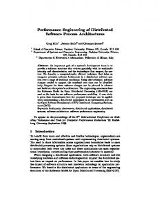
Several different Use Cases have been identified for ICAD, including Draw (draw a model) and Solve (solve a model). For this example we focus on the Draw Use Case and one particular scenario, DrawMod (Figure 1). In the DrawMod scenario, a typical model is drawn on the user’s screen. A typical model contains only nodes and beams (no triangles or plates) and consists of 2050 beams. The performance goal is to draw a typical model in 10 seconds or less.

msc DrawMod iCAD

aModel

theDatabase

new open find(modelID) retrieve(modelId) draw

close

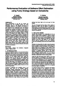
Figure 1. The DrawMod Scenario The following sections consider three alternative architectures for this application and their performance. The purpose of this case study is to illustrate the use of SPE to evaluate an application architecture and to demonstrate the importance of inter-component communication in determining performance. 5.1 Architecture 1 The first architecture uses objects to represent each beam and node. This architecture offers a great deal of flexibility, makes it possible to treat all types of elements in a uniform way, and allows the addition of new types of elements without the need to change any other aspect of the application. The Class Diagram that describes the logical view for Architecture 1 is illustrated in Figure 2. Element

Model

1..N

modelID : int beams[] : beam

Node nodeNo : int x : int y : int z : int …

draw()

Beam 2

3

elementNo : int

node1 : int node2 : int … draw()

Triangle node1 : int node2 : int node3 : int …

Plate nodes[] : node … draw()

draw()

draw() 4..N

Figure 2. Class Diagram for Architecture 1 Given the logical view in Figure 2, the DrawMod scenario expands to that in Figure 3. The unlabeled dashed arrows indicate a return from a nested set of messages. This

-9-

notation is not part of the MSC standard, it is taken from the UML [Rational Software Corporation, 1997]. The process view in Figure 4 shows that the objects in Figure 1 are each a separate process. The additional objects in Figure 3 are part of the DrawMod process corresponding to the aModel object. The Deployment Diagram illustrating the physical view in Figure 5 shows that all three processes execute on the same processor. msc DrawMod iCAD

aModel

theDatabase

aBeam

node1

node2

new draw open find(modelID) sort(beams) loop

retrieve(beam) new find(modelID, node1, node2) retrieve(node1) new retrieve(node2) new draw draw draw drawBeam

close

Figure 3. DrawMod Use Case scenario for Architecture 1 This paper illustrates model solutions using the SPE•ED™ performance engineering tool [Smith and Williams, 1997]. A variety of other performance modeling tools are available, such as [Beilner, et al., 1988], [Beilner, et al., 1995], [Goettge, 1990], [Grummitt, 1991], [Rolia, 1992], [Turner, et al., 1992]. However, the approach described here will need to be adapted for tools that do not use execution graphs as their modeling paradigm.

- 10 -

ICAD GUI

ICAD GUI

ICAD DBMS

DrawMod

«database» ICAD DBMS

DrawMod

Figure 4. DrawMod process view for Architecture 1

Figure 5. DrawMod physical view for Architecture 1

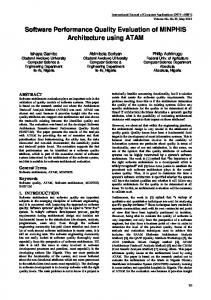
Figure 6 shows SPE•EDs screen with the execution graph corresponding to the scenario in Figure 3. The expanded nodes in the tool’s graphs are shown with color. The “world view” of the software model appears in the small navigation boxes on the right side of the screen. The top level of the model is in the top-left navigation box; its nodes are black. The top-right navigation (turquoise) contains the Initialize processing step (the steps preceding find(modelID) in the MSC). Its corresponding expanded node in the toplevel model is also turquoise. The expansion of the yellow DrawBeams processing step contains all the steps within the loop in the MSC. Note the close correspondence between the object interactions in the MSC scenario in Figure 3 and the execution graph in Figure 6. The next step is to specify software resource requirements for each processing step. The software resources we specify for this example are: • EDMS - the number of calls to the ICAD Database process • CPU - an estimate of the number of instructions executed • I/O - the number of disk accesses to obtain data from the database • Get/Free - the number of calls to the memory management operations • Screen - the number of times graphics operations “draw” to the screen The user provides values for these requirements for each processing step in the model, as well as the probability of each case alternative and the number of loop repetitions. The specifications may include parameters that can be varied between solutions, and may contain arithmetic expressions. Resource requirements for expanded nodes are in the processing steps in the corresponding subgraph. The specification of resource requirements as well as the model solutions are described in [Smith and Williams, 1997]. The parameters in this case study are based on the example in [Smith, 1990]; the specific values used are omitted here. Next, the computer resource requirements for each software resource request are specified. SPE•ED collects these specifications in an overhead matrix and stores them in its SPE database for reuse in other SPE models that execute in the environment. - 11 -

Computer resource requirements include a specification of the types of devices in the computer configuration, the quantity of each, their service times,. and the amount of processing required from each device for each type of software resource request. This configuration information is not included in current physical-view diagrams and must be obtained using supplemental SPE methods.

SPE•ED

TM

Drawmod

Software model Initialize

Drawmod

Add Find Beams

Link

Expand

Sort beams

Insert node Solve

Display:

OK

beams

Specify:

Software mod

Names

Results

Values

Overhead

Overhead

System model

Service level

SPE database

Sysmod globals

Save Scenario

Open scenario

Draw beams

Finish

©1993 Performance EngineeringServices

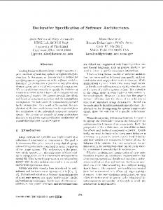
Figure 6. Execution Graph for DrawMod scenario for Architecture 1 Then, SPE•ED produces solutions for both the software execution model and the system execution model. Figure 7 shows a combination of four sets of results for the “No Contention” Solution - the elapsed time for one user to complete the Drawmod scenario with no contention delays in the computer system. This best-case solution indicates whether it is feasible to achieve performance objectives with this architecture. The solution in the top-left portion of the Figure shows that the best-case elapsed time is 992.33 seconds. The time for each processing step is next to the step. The color bar legend in the upper-right corner of the quadrant shows the values associated with each color. Values higher than the 10 second performance objective will be red, lower values are respectively cooler colors.

- 12 -

Drawmod

Draw beam < 2.70 < 5.14

Time, no contention: 992.329

< 7.57 < 10.00 ≥ 10.00

Initializ 0.272 e

< 2.59 < 5.06

Time, no contention: 0.483

< 7.53 < 10.00 ≥ 10.00

Retriev 0.121 e beam

Resource Usage Find 0.214 Beams

0.198 CPU 990.078 DEVs 2.052 Display

Sort 1.270 beams

New beam

Find 0.120 nodes

beams

Each node

Draw beam

990.512

Finish

0.060

Lock

Replace Delete

Set up node

0.241

Draw

0.001

Lock

Print

Drawmod CP Initializ DE Dis e

0.000 0.270 0.002

CP Find DE Beams Dis

0.002 0.212 0.000

CP DE Dis

0.002 1.268 0.000

< 2.50 < 5.00

Finish

Print < 2.50 < 5.00

Resource demand:

< 7.50 < 10.00 ≥ 10.00

CP Retriev DE e beam Dis

0.000 0.121 0.000

New beam

CP DE Dis

0.000 0.000 0.000

Find nodes

CP DE Dis

0.000 0.120 0.000

Model totals 0.198 CPU 990.078 DEVs 2.052 Display

beams

Draw beam

Replace Delete

Draw beam

Resource demand:

Sort beams

0.000

< 7.50 < 10.00 ≥ 10.00 Submodel totals 0.000 CPU 0.482 DEVs 0.001 Display

Each node

CP DE Dis

0.194 988.2 2.050

CP DE Dis

0.000 0.060 0.000

Lock

Set up node

Draw

Replace Delete

Print

CP DE Dis

0.000 0.241 0.000

CP DE Dis

0.000 0.000 0.001

Lock

Replace Delete

Print

Figure 7. Performance Results for Architecture 1. The “Resource usage” values below the color bar legend show the time spent at each computer device. Of the approximately 992 seconds, 990 is due to time required for I/O at the “DEVs” disk device. The DrawBeam processing step requires 991 seconds for all 2050 iterations. The time per iteration, 0.483 seconds, is in the top-right quadrant

- 13 -

along with the time for each processing step in the loop. The bottom two quadrants show the break-down of the computer device resource usage for the top level model and the DrawBeam submodel. Most of the I/O time (988 seconds) is in the DrawBeam step, the bottom-right quadrant shows that the I/O is fairly evenly spread in the submodel: 0.12 secs. for both RetrieveBeam and FindNodes, 0.24 secs. for SetUpNode. The results show that Architecture 1 clearly will not meet the performance goal of 10 seconds, so we explore other possibilities. 5.2 Architecture 2 Architecture 1 uses an object for each beam and node in the model. While this provides a great deal of flexibility, using an object for each node and beam is potentially expensive in terms of both run-time overhead and memory utilization. We can reduce this overhead by using the Flyweight pattern [Gamma, et al., 1995]. Using the Flyweight pattern in ICAD allows sharing of beam and node objects and reduces the number of each that must be created in order to display the model. Each model now has exactly one beam and node object. The node and beam objects contain intrinsic state, information that is independent of a particular beam or node (such as coordinates). They also know how to draw themselves. Extrinsic state, coordinates and other information needed to store the model are stored separately. This information is passed to the beam and node flyweights when it is needed. The Flyweight pattern is applicable when [Gamma, et al., 1995]: • the number of objects used by the application is large, • the cost of using objects is high, • most object state can be made extrinsic, • many objects can be replaced by fewer, shared objects once the extrinsic state is removed, and • the application does not depend on object identity. The SPE evaluation will determine if the ICAD application meets all of these criteria. Instead of using an object for each Beam and Node, we use a shared object based on the Flyweight pattern. The state information is removed from the Beam and Node classes and is stored directly in Model. The Class Diagram for this approach is shown in Figure 8. The scenario resulting from this set of classes is shown in Figure 9. As shown in Figure 9, constructors for Node and Beam are executed only once, resulting in a savings of many constructor invocations. This architecture change has a minor effect on the process view, and no effect on the physical view. The beam and node objects are still part of the DrawMod process, now

- 14 -

there is only one of each. In the physical view, the three processes are still assigned to the same processor. Element

Model 1..3 modelID : int beams[] : Points

Node

draw()

Beam

nodeNo : int x : int y : int z : int …

elementNo : int

node1 : int node2 : int … draw()

Triangle node1 : int node2 : int node3 : int …

Plate nodes[] : node … draw()

draw()

draw()

Figure 8. Class Diagram for Architecture 2

msc DrawMod iCAD

aModel

theDatabase

aBeam

aNode

new new new draw open find(modelID) sort(beams) loop

retrieve(beam) find(modelID, node1, node2) retrieve(node1) retrieve(node2) draw(point1) draw(point2) draw(point1, point2) close

Figure 9. DrawMod Use Case Scenario for Architecture 2 The changes to the execution graph for this architecture are trivial. The graph nodes corresponding to the “New” processing steps move from the yellow subgraph that represents the DrawBeam processing step to the turquoise subgraph corresponding to the Initialize processing step. This takes the corresponding resource requirements out of the loop that is executed 2050 times.

- 15 -

Drawmod rev1

Time, no contention: 992.267

< 2.70 < 5.14

Initialize

< 7.57

0.272

< 10.00 ≥ 10.00 Resource Usage

Find Beams

0.214

0.137 CPU 990.078 DEVs 2.052 Display

Sort beams

1.270

beams

Draw beam

Finish

990.450

0.060

Lock

Replace

Delete

Print

Figure 10. Results for DrawMod scenario for Architecture 2 The overall response time is reduced from 992.33 to 992.27 seconds. The results of the software execution model for this approach indicate that using the Flyweight pattern did not solve the performance problems with ICAD. Constructor overhead is not a significant factor in the DrawMod scenario. The amount of constructor overhead used in this case study was derived from a specific performance benchmark and will not generalize to other situations. It is compiler, operating system, and machine dependent; in our case constructors required no I/O. It is also architecture-dependent; in our example there is no deep inheritance hierarchy. It is also workload-dependent;

- 16 -

in this case the number of beams and nodes in the typical problem is relatively small. Nevertheless, we choose to retain the Flyweight approach; it will help with much larger ICAD models where the overhead of using an object for each beam and node may become significant, making the architecture more scalable. The evaluation of Architecture 2 illustrates two important points: modifying performance models to evaluate alternatives is relatively easy; and it is important to quantify the effect of software alternatives rather than blindly follow a “guideline” that may not apply. Note that the relative value of improvements depends on the order that they are evaluated. If the database I/O and other problems are corrected first, the relative benefit of flyweight will be larger. The problem in the original design, excessive time for I/O to the database, is not corrected with the Flyweight pattern, so the next architecture focuses on reducing the I/O time due to database access. 5.3 Architecture 3 This architecture uses an approach similar to Architecture 2 (Figure 8) but modifies the database management system with a new operation to retrieve a block of data with one call: retrieveBlock() . Architecture 3 uses this new operation to retrieve the beams and nodes once at the beginning of the scenario and stores the data values for all beams and nodes with the model object rather than retrieve the value from the database each time it is needed. This new operation makes it possible to retrieve blocks containing 20K of data at a time instead of retrieving individual nodes and beams 3. A single block retrieve can fetch 64 beams or 170 nodes at a time. Thus, only 33 database accesses are required to obtain all of the beams and 9 accesses are needed to retrieve the nodes. The class diagram for Architecture 3 does not change from Architecture 2. Figure 11 shows the MSC that corresponds to the new database access protocol. The bold arrows indicate messages that carry large amounts of data in at least one direction. Although this notation is not part of the MSC standard, we have found it useful to have a way of indicating resource usage on scenarios that are intended for performance evaluation. The logical, process, and physical views are essentially unchanged; the only difference is the new database operation, retrieveBlock() . Figure 12 shows the execution graph corresponding to Figure 11 along with the results for the “No Contention” solution. The time for Architecture 3 is approximately 8 seconds – a substantial reduction.

3

Note: A block size of 20K is used here for illustration. The effect of using different block sizes could be evaluated via modeling to determine the optimum size.

- 17 -

Other improvements to this architecture are feasible, however, this serves to illustrate the process of creating software execution models from architecture documents and evaluating trade-offs. It shows that it is relatively easy to create the initial models, and the revisions to evaluate alternatives are straightforward. The simple software execution models are sufficient to identify problems and quantify the performance of feasible alternatives. Software execution models also support the evaluation of different process compositions and different assignments of processes to physical processors. Once a suitable architecture is found, SPE studies continue to evaluate design and implementation alternatives. msc DrawMod iCAD

aModel

theDatabase

aBeam

aNode

new new new draw open find(modelID) loop

retrieveBlock(beams) find(nodes)

loop

loop

retrieveBlock(nodes) match

draw(point1) draw(point2) draw(point1, point2) close

Figure 11. DrawMod scenario for Architecture 3 Analysts will typically evaluate other aspects of both the software and system execution models to study configuration sizing issues and contention delays due to multiple users of a scenario and other workloads that may compete for computer system resources. In these additional performance studies, the most difficult aspect has been getting reasonable estimates of processing requirements for new software before it is created. The SPE process described here alleviates this problem. Once this data is in the software performance model, the additional studies are straightforward and are not described here. Information about these additional performance models is in [Smith and Williams, 1997].

- 18 -

SPE•ED

TM

Results screen

Drawmod design 3

Time, no contention: 7.964

< 2.81 < 5.21

Initialize

< 7.60

0.412

< 10.00

Solution:

≥ 10.00

View:

No contention

Residence time

Contention

Rsrc demand

System model

Utilization

Adv sys model

SWmod specs

Resource Usage

Get data

5.440

0.003 CPU 5.908 DEVs 2.052 Display

Each beam Simulation data Pie chart

Solve

Display:

OK

Specify:

Software mod

Names

Results

Values

Overhead

Overhead

System model

Service level

SPE database

Sysmod globals

Save Scenario

Open scenario

Match and draw

Close DB

©1993 Performance EngineeringServices

2.051

0.060

Lock

Replace

Delete

Print

Figure 12. Execution Graph for DrawMod scenario for Architecture 3. 6. Summary and Conclusions This paper presents and illustrates the SPE process for software architecture evaluations. We demonstrated that software execution models are sufficient for providing quantitative performance data for making many architecture trade-off decisions. Other SPE models are appropriate for evaluating additional facets of architectures and more detailed models of the execution environment. Kruchten’s “4+1” view model is a useful way of thinking about the information required to completely document a software architecture. Our experience is that, at least from a performance perspective, each view is not atomic. Each of the views, particularly the process view and the physical view, will likely have several possible sub-views to represent information at different levels of abstraction. The current SPE process obtains information from available documentation and supplements it with information from performance walkthroughs and measurements. Initially the SPE process was ad-hoc and informal. Both the information requirements and the SPE evaluation process are now better defined [Williams and Smith, 1995], so

- 19 -

it makes sense to extend the architecture documentation to include SPE information to make automation of these steps viable. The additional information required includes resource requirements for processing steps, and computer configuration data. Most diagrams really serve as documentation of architecture and design decisions and do not support making those decisions. We need notations, with tool support, that provide decision support as well as documentation. (Use Case scenarios are an exception to this, which may account for their rapid acceptance and current popularity). In particular, both the process view and the physical view contain facts that are best produced from performance studies (e.g., the assignment of objects to processes and assignment of processes to processing components). Current diagrams for these views are rather complex and it doesn’t make sense to create them before the SPE study is executed, because labor-intensive changes may be required. We envision a tool that would display processes and processing components and give the user a direct-manipulation interface to drag and drop processes to processors (and objectsmethods to processes in the logical view), automatically create and solve performance models, give users quantitative feedback on each alternative, then produce processview and physical-view diagrams as output once the user has picked the mapping they desire. The case study results verify the earlier observation that “performance is largely a function of the frequency and nature of inter-component communication.” The case study also demonstrates that SPE models are sufficient to identify architectures with suitable inter-component communication patterns. 7. References [Abowd, et al., 1993] G. Abowd, R. Allen, and D. Garlan, "Using Style to Understand Descriptions of Software Architecture," Software Engineering Notes, vol. 18, no. 5, pp. 9-20, 1993. [Baldassari, et al., 1989] M. Baldassari, B. Bruno, V. Russi, and R. Zompi, "PROTOB: A Hierarchical ObjectOriented CASE Tool for Distributed Systems," Proceedings of the European Software Engineering Conference, 1989, Coventry, England, September, 1989. [Baldassari and Bruno, 1988] M. Baldassari and G. Bruno, "An Environment for Object-Oriented Conceptual Programming Based on PROT Nets," in Advances in Petri Nets, Lectures in Computer Science No. 340, Berlin, Springer-Verlag, 1988, pp. 1-19. [Beilner, et al., 1988] H. Beilner, J. Mäter, and N. Weissenburg, "Towards a Performance Modeling Environment: News on HIT," Proceedings of the 4th International Conference on Modeling Techniques and Tools for Computer Performance Evaluation, Plenum Publishing, 1988.

- 20 -

[Beilner, et al., 1995] H. Beilner, J. Mäter, and C. Wysocki, "The Hierarchical Evaluation Tool HIT," in Performance Tools and Model Interchange Formats, F. Bause and H. Beilner, ed., Dortmund, Germany, Universität Dortmund, Fachbereich Informatik, 1995, pp. 6-9. [Booch, 1994] G. Booch, Object-Oriented Analysis and Design with Applications, Redwood City, CA, Benjamin/Cummings, 1994. [Booch, 1987] G. Booch, Software Engineering with Ada, Second Edition, Menlo Park, Benjamin/Cummings, 1987.

CA,

[Buhr and Casselman, 1996] R. J. A. Buhr and R. S. Casselman, Use Case Maps for Object-Oriented Systems, Upper Saddle River, NJ, Prentice Hall, 1996. [Buhr and Casselman, 1994] R. J. A. Buhr and R. S. Casselman, "Timethread-Role Maps for Object-Oriented Design of Real-Time and Distributed Systems," Proceedings of OOPSLA '94: Object-Oriented Programming Systems, Languages and Applications, Portland, OR, October, 1994, pp. 301316. [Buhr and Casselman, 1992] R. J. A. Buhr and R. S. Casselman, "Architectures with Pictures," Proceedings of OOPSLA '92: Object-Oriented Programming Systems, Languages and Applications, Vancouver, BC, October, 1992, pp. 466-483. [Clements, 1996] P. C. Clements, "Coming Attractions in Software Architecture," Technical Report No. CMU/SEI-96-TR-008, Software Engineering Institute, Carnegie Mellon University, Pittsburgh, PA, Jaunary, 1996. [Clements and Northrup, 1996] P. C. Clements and L. M. Northrup, "Software Architecture: An Executive Overview," Technical Report No. CMU/SEI-96-TR-003, Software Engineering Institute, Carnegie Mellon University, Pittsburgh, PA, February, 1996. [Gamma, et al., 1995] E. Gamma, R. Helm, R. Johnson, and J. Vlissides, Design Patterns: Elements of Reusable Object-Oriented Software, Reading, MA, Addison-Wesley, 1995. [Garlan and Shaw, 1993] D. Garlan and M. Shaw, "An Introduction to Software Architecture," in Advances in Software Engineering and Knowledge Engineering, Volume 2, V. Ambriola and G. Tortora, ed., Singapore, World Scientific Publishing, 1993, pp. 1-39.

- 21 -

[Goettge, 1990] R. T. Goettge, "An Expert System for Performance Engineering of Time-Critical Software," Porceedings of the Computer Measurement Group Conference, Orlando, FL, 1990, pp. 313-320. [Grummitt, 1991] A. Grummitt, "A Performance Engineer's View of Systems Development and Trials," Proceedings of the Computer Measurement Group Conference, Nashville, TN, 1991, pp. 455463. [Hrischuk, et al., 1995] C. Hrischuk, J. Rolia, and C. M. Woodside, "Automatic Generation of a Software Performance Model Using an Object-Oriented Prototype," Proceedings of the Third International Workshop on Modeling, Analysis, and Simulation of Computer and Telecommunication Systems, Durham, NC, January, 1995, pp. 399-409. [ITU, 1996] ITU, "Criteria for the Use and Applicability of Formal Description Techniques, Message Sequence Chart (MSC)," International Telecommunication Union, 1996. [Jacobson, et al., 1992] I. Jacobson, M. Christerson, P. Jonsson, and G. Overgaard, Object-Oriented Software Engineering, Reading, MA, Addison-Wesley, 1992. [Kazman, et al., 1996] R. Kazman, G. Abowd, L. Bass, and P. Clements, "Scenario-Based Analysis of Software Architecture," IEEE Software, vol. 13, no. 6, pp. 47-55, 1996. [Kazman, et al., 1997] R. Kazman, M. Klein, M. Barbacci, T. Longstaff, H. Lipson, and J. Carriere, "The Architecture Tradeoff Analysis Method," Software Engineering Institute, Carnegie Mellon University, Pittsburgh, PA, 1997. [Kruchten, 1995] P. B. Kruchten, "The 4+1 View Model of Architecture," IEEE Software, vol. 12, no. 6, pp. 42-50, 1995. [Perry and Wolf, 1992] D. E. Perry and A. L. Wolf, "Foundations for the Study of Software Architecture," Software Engineering Notes, vol. 17, no. 4, pp. 40-52, 1992. [Rational Software Corporation, 1997] Rational Software Corporation, "Unified Modeling Language: Notation Guide, Version 1.1," Rational Software Corporation, Santa Clara, CA, September, 1997. [Rolia, 1992] J. A. Rolia, "Predicting the Performance of Software Systems," Ph.D. Thesis, University of Toronto, 1992.

- 22 -

[Rumbaugh, et al., 1991] J. Rumbaugh, M. Blaha, W. Premerlani, F. Eddy, and W. Lorensen, Object-Oriented Modeling and Design, Englewood Cliffs, NJ, Prentice Hall, 1991. [Smith, 1990] C. U. Smith, Performance Engineering of Software Systems, Reading, MA, Addison-Wesley, 1990. [Smith and Williams, 1998] C. U. Smith and L. G. Williams, "Software Performance Engineering for Object-Oriented Systems: A Use Case Approach," submitted for publication, 1998. [Smith and Williams, 1997] C. U. Smith and L. G. Williams, "Performance Engineering Evaluation of ObjectOriented Systems with SPEED," in Computer Performance Evaluation: Modelling Techniques and Tools, Lecture Notes in Computer Science, vol. 1245, R. Marie, B. Plateau, M. Calzarossa and G. Rubino, ed., Berlin, Springer-Verlag, 1997, pp. 135-154. [Smith and Williams, 1993] C. U. Smith and L. G. Williams, "Software Performance Engineering: A Case Study Including Performance Comparison with Design Alternatives," IEEE Transactions on Software Engineering, vol. 19, no. 7, pp. 720-741, 1993. [Turner, et al., 1992] M. Turner, D. Neuse, and R. Goldgar, "Simulating Optimizes Move to Client/Server Applications," Proceedings of the Computer Measurement Group Conference, Reno, NV, 1992, pp. 805-814. [Williams and Smith, 1995] L. G. Williams and C. U. Smith, "Information Requirements for Software Performance Engineering," in Quantitative Evaluation of Computing and Communication Systems, Lecture Notes in Computer Science, vol. 977, H. Beilner and F. Bause, ed., Heidelberg, Germany, Springer-Verlag, 1995, pp. 86-101.

- 23 -