Performance Expectations on Ada Programs Göran Wall, Lars Asplund, Lars Björnfot and Kristina Lundqvist Department of Computer Systems, Uppsala University P.O. Box 325, S–751 05 Uppsala, Sweden E–mail:
[email protected] Tel: +46 18 18 10 09 Fax: +46 18 55 02 25
Abstract.A method for performance estimation of Ada programs by analyzing their syntactical structure is presented. The use of algorithmic knowledge by means of code annotations to improve the analysis is discussed. Dual loop benchmarks are used to estimate the execution time for basic Ada features from which all other estimationsare derived. An example program is analyzed and compared to its actual time showing an initial overestimation of 40%. It is suggested that the method is integrated with the Ada–environment to ensure that estimations are consistent with the current version of the code.
1
Introduction
Much work [1], [2], [3], [4], [5] has been done in the fields of performance evaluation or analysis of temporal behavior of Ada–programs. The work follow three different directions, synthetic benchmarks, feature benchmarks and analytical methods. There are two kinds of synthetic benchmarks, programs that represent a particular domain of computation and specific applications. These benchmarks are good for making comparisons between different compilers and architectures. Examples of the first kind of benchmark are [1], which models typical mathematical computations, and [2], which models a typical program with respect to the distribution of different types of statements. Application benchmarks are programs that solve specific problems. They are suitable for comparing programs, written in different languages, solving the same problem. Feature benchmarks isolate and measure the time it takes to execute a specific language construct, for example procedure call and return overhead for a procedure with no parameters or the minimum time required for doing a rendezvous in Ada. Examples of this type of benchmarks can be found in [3] and [4]. The benchmarks can be used to evaluate how well a given compiler and architecture deals with specific Ada features. The last kind of benchmark are based on analytical methods, which may be integrated with some software CAD. An example of this is CAEDE [5] which is a design tool that can analyze structure and interactions of a program design with respect to execution time. This makes it easier to detect flaws in a design at an earlier stage which could have an adverse effect on performance. None of the approaches discussed above (all of which are very valuable in their own way) enables a programmer to evaluate the performance of a specific program. To
obtain it one have to use some profiling tool/technique that measures the time it takes to execute different parts of a program. A common method for performance measurement is to write a special program, a test bed, from where the part/parts to be measured are called from. The writing of test beds take a lot of time from the programming task at hand. It can also be the case that profiling is impossible because of incomplete programs and lack of data. One possible solution is to estimate the execution time for a program by examining its components. This eliminates the need to actually execute a program and makes it possible to examine the interesting parts as they are. The problem of lack of data can also be overcome. Even if the actual data to be processed is not available, knowledge of how it is organized must be known in order to write programs. Knowledge of how the data is organized and of how it is to be processed, ie. algorithmic knowledge, is combined with information about how long time it takes to execute different basic Ada features. This enables an estimation of how fast some execution thread of a program will execute. Two examples where static performance analysis of programs are applied to source level C–programs are [8] and [9]. The main difference between the two approaches is how timing information is collected for simple language constructs. In [8] the actual assembler code produced by the compiler is used whereas in [9] one tries to predict how code would be generated by the intended.
2
Overview
In order to derive performance estimations for programs from their components, some set of basic (smallest) language features has to be identified and evaluated with respect to execution time. The evaluation technique should be compiler and architecture independent in order to improve the portability of an analysis tool. Programs in general do not contain enough information to be analyzable, therefore, algorithmic knowledge must be supplied with the code to make possible and improve the analysis. One aspect of the analysis is correctness. Important questions like; How far from the real execution time lies the estimate? Can one be sure that two estimates a and b of two different versions of some code express the true difference in execution time between the versions? Might it not be the case that b is slower than a but the analysis of b gave a more accurate estimate? Generally this can be impossible to answer, but if b meets the deadline and a does not, it does not matter if b is slower than a. The issue of correctness will not be discussed.
3
Language Features
To determine the language features to consider in an analysis the relevant components of the language must first be identified and studied. The components of Ada, as in Pascal–like languages, can be classified into three major syntactical groups: declarations, statements and expressions. Each of the three groups has some unique properties. Generics is a thing that complicates the matter. There are two ways of implementing generics, code sharing and macro expansion. The difference from a performance point
of view is where the extra overhead lies. If code sharing is used the overhead is incurred at run–time and if macro expansion is used at compile–time. 3.1
Declarations
Declarations introduce new objects. The objects can be of various kinds such as types, variables, tasks, subprograms etc.. Most declarations can be resolved by the compiler and require little or no processing during program execution. Declarations involving initializing expressions on the other hand must be considered. Another thing of interest is type definitions. Both derived types and subtypes gives information on the amount of data being moved in an assignment statement. Subtypes also gives some information when constraint checks are not needed. 3.2
Statements
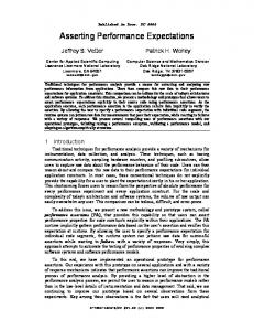
Statements are the means that exist to manipulate the storage and move the computation forward. There are many types of statements in Ada. One way of classifying the statements of Ada is given in [6] as shown in figure 1. Statement
Simple
Sequential null assignment procedure call entry call code delay abort
Compound
Control exit goto raise return
Sequential if case loop block
Parallel accept select
Fig. 1. A classification of Ada statements.
Statements of obvious interest are, in the simple sequential group, assignment, procedure call, entry call and delay. Code statements are highly machine dependent and are therefore difficult to say something meaningful about. Things important here are the time required to store a datum of a given type at some location, procedure call and return overhead and what impact parameters have on procedure calls. One tricky thing that can occur in this group are directly recursive and mutually recursive procedures. If recursion is to be analyzed some way to express the maximum depth of recursive calls must be devised. In the simple control group the purpose of the statements is to move the thread of execution elsewhere. With the exception of the exit statement, which can have a conditional expression associated with it whose evaluation time is significant, this group of statements add little to the execution time of a program.
Statements in the compound sequential group are more complicated. The block statement can be treated as a procedure without procedure call/return and parameter passing overhead. The if and case statements are similar. Both select a sequence of statements to execute depending on the value of some expression. The problem is, since the value of the expression is not known, to know which sequence of statements is chosen. The loop statement can be expressed in different ways. While loops and unbounded loops makes it difficult to predict the number of iterations of the enclosed statements and that have to be dealt with in some way. The last group are the compound parallel statements accept and select. Since this method only estimates single thread execution, many aspects of the tasking system can be ignored. Under this limitation, select and accept statements behave like conditional statements. The overhead in a rendezvous plus time for parameter passing are factors to take into account. Restrictions. To make possible and simplify the analysis of how many times the flow of control passes a particular point the following restrictions on programs are made:
3.3
S
Goto statements, for obvious reasons, are not allowed.
S
Recursion is not allowed.
S
All loops must be bounded, ie. the maximum number of iterations of a loop must be derivable either from the range of the loop or from an annotation.
Expressions
Since we are not going to execute any programs, the actual value of an expression becomes irrelevant. What is relevant is the type of the resulting expression and the way in which it is computed. Expressions are treated differently depending on in which context they appear. The result of composite type expressions are always copied in assignments but may be passed by reference in a subprogram call. Scalars are always copied. Expressions can be arbitrarily complex and consist of many sub expressions. The sub expressions are either defined by a programmer or by the predefined language environment, such as arithmetics on natural numbers. This is a reason to study them separately.
4
Measurements
As mentioned earlier, a basic set of feature benchmarks is used to derive estimations for larger program constructs. This set should contain benchmarks that deal with the constructs discussed in section 3. Other obvious candidates for benchmarks are the operations given in the predefined language environment, package standard etc.. The execution time for language features can be partitioned into two parts, one constant–time part and one variable–time part. As an example of a constant–time part, consider the fact that an if statement always have to test a boolean value and make a jump based on the result of the test. The variable–time part of the if statement consists
of the evaluation of the conditional expression to a truth–value and the execution of the statements of the then part. The constant–time part will here after be referred to as the overhead of a statement. The overhead can be parameterized with respect to some relevant properties, as is the case with assignments and subprogram parameters. There are evidence ,[3] and [4], that the dual loop technique is useful for establishing statement overhead, although [7] show examples of timing variations in the technique. These variations will of course affect the accuracy of any performance estimation method based on the dual loop technique and therefore speaks against using it. Still, the method being described is approximate and the advantage of having a portable method for establishing statement overhead is appealing. start := clock; –– Control Loop null_loop: for i in 1 .. nr_iterations loop Trick_Optimizer; end loop null_loop; stop := clock; null_loop_overhead := stop – start; start := clock; –– Test Loop feature_loop: for i in nr_iterations loop Trick_Optimizer; feature; end loop feature_loop; stop := clock; feature_loop_overhead := stop – start; feature_overhead := (feature_loop_overhead – null_loop_overhead) / nr_iterations; Fig. 2. The principle of the Dual–loop technique.
Benchmarks using the dual loop technique must be designed in a way that minimize the dynamics of the feature being measured so as to assure an as accurate estimation as possible.
5
A Timing Schema
Having established a set of basic benchmarks for determining overhead for Ada constructs some method must be applied to derive estimations for larger constructs. The principles for a timing schema describing this are illustrated by using some fundamental Ada–statements.
Most statements are simple to estimate since the time it takes to execute can be derived by adding up the estimations of their components. The following notation will be used:
5.1
S
V, E, S and P are meta variables denoting arbitrary variables, expressions, statements and subprograms.
S
O, possibly parametrized, denotes a feature overhead.
S
E denotes the estimation function.
S
T is a function from expressions to types.
S
M is a function from positional parameters to modes.
S
B is a function from subprogram identifiers to subprogram bodies.
Assignments
Assignment is the corner stone in the imperative programming model. The store is modified by repeated assignments until some final state is achieved and the answer can be extracted from it. (Eqn 1) E[V :+ E] + O assign[T(V)] ) E[E] 5.2
Subprograms
Subprograms, procedures, functions and entry calls can in principle be treated the same with the difference being the size of the overhead, O Subprogram. For example, the estimation of a procedure call is done like equation 2 below. Where O proc is procedure call/return overhead for a parameterless procedure, O param[T(pi), M(p i)] is the parameter passing overhead generated by a parameter of type T(p i) and mode M(p i), E[p i] is the estimated execution time for evaluating p i and E[B(P)] is the estimated execution time for the body of procedure P. (Eqn 2) N
E[P(p 0, . . . , pN)] + O proc )
ȍ(E[p ] ) O i
[T(p i), M(pi)]) ) E[B(P)]
param
i+0
5.3
Sequential Compound Statements
As mentioned in section 3 the compound statements are more complex and harder to estimate since they introduce a choice of what execution thread to follow next (if, case) or how many times the body of a loop (for, while) should be executed. To illustrate the principle the timing schema for a simple if statement and a for statement are given. An if statement not executing within a loop is analyzed as given in equation 3. This makes sense since it is only executed once within that context. If it is executed within a loop equation 3 gives a very pessimistic estimation, but it is the best possible if no knowledge about the number of times each branch is entered is available.
(Eqn 3) E[If E Then S 0 Else S 1 End If] + Oif ) E[E] ) max(E[S 0], E[S1]) A for loop have a more complicated kind of overhead which consists of two parts, initialization overhead and revolution overhead (increment and test). If it is not possible to derive the number of iterations from the Iteration_Scheme some external information must be supplied in order to do a meaningful analysis. (Eqn 4) E[for I in Iteration_Scheme loop S End loop] + O init ) O rev )
ȍ(S ) O
) where
rev
i
i is derivable from Iteration_Scheme However, it is hard to separate the two kinds of overhead with the dual loop technique and as a consequence the initialization part may become a part of the revolution overhead. It is obvious that, the more iterations performed in a loop the less the initialization overhead contributes to its total execution time.
6
Reinforcing the Timing Schema with Algorithmic Knowledge
Programs in general does not contain enough information about the applied algorithm to allow good predictions about the flow of control. Therefore, some way of annotating programs with this information is required. There are two kinds of annotations, flow annotations and parameter annotations. Flow annotations capture how different parameters (program variables) influence the flow of control and parameter annotations quantifies these parameters ie. put a bound on what values they may assume. As an example, consider a situation where 3 3 matrixes have to be multiplied. Either a custom 3 3 multiplier or a general multiplier is written. In the first case we know exactly how many iterations are needed and it can be specified directly in the code with flow annotations. In the latter case, the dimension of the matrix is not known until the point where the multiplier is actually called, thus limiting the use of flow annotations to describing how the computation depends on its dimensions. At the point of call parameter annotations have to be used to specify the actual dimensions of the matrix. 6.1
Flow Annotations
The purpose of flow annotations is to mark how many times a certain point in the code will be passed or how many iterations, maximally, a loop will iterate. In [8] several useful ways of annotating programs with application specific information to improve predictions about the flow of control are described (bounded loops, scopes, markers and loop–sequences). These annotations are integrated with the programming language being used, which is a version of C. This requires modification of the C compiler. Doing the same with Ada is, since Ada is standardized, out of the question. Instead, a convention based on comments will be used. The annotations can be adopted with some modifications.
Description of Flow Annotations. For more precise definitions of the following concepts see [8]: S
A bounded loop is a loop where the loop construct have been annotated with the maximum possible iterations it may iterate
S
A scope defines a region of code. Scopes coincides with the loop construct.
S
A marker defines how many times, maximally, the flow of control will pass the marked point. Markers must lay within a scope.
S
A loop–sequence is a sequence of mutually dependent loops where the total number of iterations is less than the sum of the iterations of the single loops.
Instead of giving a number in the bounded loop and marker annotations a time bound can be given. This is particular valuable when dealing with process communication, I/O etc., where the time consumption lies outside the scope of this method of analysis. These time bounds can be used to facilitate a top–down program developing style. Language constructs with time bounds need not be analyzed further and it relieves the programmer from having to write all of the code before making an analysis. The nature of Adas tasking leads to the use of the following construct in order to allow the task to live on. loop select –– A lot of entries end select; end loop; This construct clearly conflicts with the restriction that all loops must be bounded. Fortunately it gets the job done in one iteration and therefore it is reasonable to introduce a cyclic annotation marking it as a distinguished loop construct. 6.2
Parameter Annotations
Unfortunately application specific information can not always be supplied at the time of writing the code. This is not surprising since much of the code written in a system is intended to operate on some data type/structure and several different instances of it will exist. Typically the execution time of a subprogram depend on one or more of its parameters. Flow annotations can describe how the parameters influence the computation without knowledge of the values the parameters can assume, but these values must be supplied at some point in order to perform the analysis. The purpose of parameter annotations is to request application specific information about subprogram parameters at the point of subprogram call so that the subprogram can be estimated. Defining a reasonable set of these annotations is not easy since information about the implementation of a subprogram can not be given away. Therefore these annotations must capture the nature of the types in Ada and abstract data structures in general.
Iteration. Typically a loop construct iterate a number of times as determined by some constants (lower and upper bound) or iterate over some data structure in which case the number of elements determines the bound. For the number of elements to be meaningful the data structure operated on must have some function or attribute that gives it meaning. For example, lists have length, sets have cardinality and arrays have one or more dimensions of some length. This suggests the following annotations: S
Max defines the maximum value of some variable.
S
Min defines the minimum value of some variable.
S
Card defines the number of elements of some variable.
Unfortunately iterations where the stop conditions, of the kind below, are very common and it is not clear at this point how handle it. while Delta t Threshold loop –– Statements calculating Delta end loop; In the following example the definition and use of parameter annotations is illustrated. Note that there can be different calls to the function Fac with different instantiations of the parameter annotation. –– Function specification with a parameter annotation. ––| Max(N => ?) function Fac(N : Integer) return Integer; –– Function call with instantiation of the parameter –– annotation ––| Max(N => 10) F := Fac(X);
7
An Example
The following is an estimation of the execution time of the bubble sort program seen in figure 3. The basic set of benchmarks were built using tests from the PIWG suite and some other tests built using templates provided with suite. The estimations given here have been calculated by hand. The bubblesort package consists of one public procedure and one local procedure. Since all algorithmic information needed for an estimation is present in the program there is no need of annotations. 7.1
Procedure Swap
The procedure takes two integer type parameters with mode in out. One local variable of type integer is allocated but not initialized so it is ignored, see equation 5. In the body
with Types; use Types; package Bubble_Sort is procedure Sort(Numbers: in out Number_Vector); end Bubble_Sort; package body Bubble_Sort is procedure Swap(X, Y: in out Integer) is Tmp : Integer; begin Tmp := X; X := Y; Y := Tmp; end Swap; procedure Sort(Numbers: in out Number_Vector) is begin for I in Natural range 1 .. (Numbers’Last – 1) loop for J in Natural range 1 .. (Numbers’Last – I) loop if Numbers(J) > Numbers(J + 1) then Swap(Numbers(J), Numbers(J+1)); end if; end loop; end loop; end Sort; end Bubble_Sort; Fig. 3. A bubblesort program
of the procedure three integer assignments are made, see equation 6. The equations for array indexing and arithmetics are omitted for sake of space. (Eqn 5) E[Swap(X, Y)] + O proc ) E[X] ) E[Y] ) O param[T(X), M(X)] ) O param[T(Y), M(Y)] ) E[B(Swap)] where X + Numbers(J) and Y + Numbers(J ) 1) (Eqn 6) E[B(Swap)] + 3
Oassign[Integer]
Substituting measured values, obtained using the methods named in beginning of section 6, for the overhead terms in equations 5 and 6 gives E[Swap(X, Y)] + 2 . 7 ms as an estimation for one call of procedure Swap.
7.2
Procedure Sort
Procedure Sort takes one argument of type Number_Vector of mode in out. The execution of the inner loop in the procedure depends on the outer one. The range of the the two loops can easily be derived from the definition of the type Number_Vector. Observe that no constraint checks are needed. Only the inner loop is shown below, see equation 7. As mentioned before the simplified overhead for for loops have been used. (Eqn 7) E[for J in R loop S end loop] +
ȍ(E[S] ) O
loop
) where
J
R + Natural range 1 .. Number_VectorȀLast and S + if Numbers(J) u Numbers(J ) 1) then Swap(Numbers(J), Numbers(J ) 1)) end if (Eqn 8) E[if X u Y then Swap(X, Y) end if] + O if ) E[X u Y] ) E[Swap(X, Y)] where X + Numbers(J) and Y + Numbers(J ) 1) 7.3
Results
Substituting measured values for the overhead terms in the equations above, taking the outer loop sum over equation 7, with 10000 iterations, and adding overhead for calling Sort yields the execution time estimation 209.0 s. For comparison the program where actually run on tree different sets of data, one randomly unordered (U), one sorted in reverse order (R) and one sorted (S). The measured execution times were, (U) 140.0 s, (R) 150.0 s and (S) 134.0 s. The relative closeness of the times (U) and (R) suggests that the array variables occurring both in the if statement and the call to the Swap procedure only are evaluated once. Recalculating the estimation of procedure Swap with this assumption yields a much closer result of 181.0 s which is an over estimation of (R) by only 18% instead of 40% with the earlier result.
8
Future Work
An attractive environment for a first implementation of a performance tool based on the principles in this paper is Rationals. Using the LRM–interface built on the DIANA representation of Ada units, it is easy to traverse the syntax tree of a program. Currently our aim is to implement a tool for a subset of Ada. This tool will be a platform for expanding and refining the concepts given here. The implementation will be done in the Rational environment. The subset of Ada that will be considered is as follows: The types boolean, integer and float and the operations on them as defined in package standard. In addition the statements, for–loop, :=, if–then–else, procedure call and function call will be included.
The phase under which a static performance analysis tool has its greatest potential value is the coding phase. Code change quickly during this phase and the need of quick appraisals of the execution speed of new coding solutions is greater than estimating whole programs. Also, in large systems not all parts are time critical. This implies some desirable properties that a tool should have: Incremental analysis. The tool should be able to handle incremental analysis, ie. results from imported units propagate up to higher levels and need not be recalculated. This corresponds to a bottom–up development. The top–down development is handled implicitly. Library integration. The results from code analysis should be coupled with the version of the analyzed code. This enables detection of the fact that the timing behavior may have changed in higher layers of the program. Interactive. The tool should be callable from within the program editing facility being used. Thus allowing instant analysis of small portions of code. Figure 4 shows one possible configuration of a design environment. The different comAnnotated programs Ada–library
Ada benchmarks
Library Manager
Performance analysis
Programmer interaction Estimations Fig. 4. Sketch of design environment.
ponents in figure 4 are; Ada–library – the collection of annotated Ada–units. Library Manager – the library manager extended with the function of keeping track of invalidation of the performance describing units. Ada benchmarks – a database with Ada feature benchmarks. Performance Analysis Tool – an interactive analysis tool.
9
References [1]
H.J. Curnow and B.A. Wichman A Synthetic Benchmark. Computer Journal 19(1):43–49, January 1976
[2]
R.P. Weicker Dhrystone: A Synthetic Systems Programming Benchmark. Communications of the ACM, 27(10):1013–1030, October 1984.
[3]
R.M. Clapp, L.Duchesnea , R.A. Voltz, T.N. Mudge and T. Schultze Toward Real–Time Performance Benchmarks For Ada Communications of the ACM, 29(8):760–778, August 1986.
[4]
Ada Letters Special Edition from the SIGAda Performance Issues Working Group on Ada Performance Issues, X(3) Winter 1990.
[5]
C.M. Woodside, E.M. Hagos, E. Neron and R.J.A. Buhr The CAEDE Performance Analysis Tool. Proceedings of the First Symposium on environments and Tools for Ada, XI(3) Spring 1991.
[6]
J.G.P. Barnes Programming in Ada, 3rd edition. Addison–Wesley, 1989.
[7]
N. Altman and N. Weiderman Timing Variations in Dual Loop Benchmarks. Technical Report CMU/SEI–87–TR–21, SEI, CMU.
[8]
Caculating the Maximum Execution Time of Real–Time Programs, P. Puschner and Ch. Koza. Real–Time Systems, 1(2):159––176, Sep. 1989.
[9]
Experiments with a Program Timing Tool Based on Source–Level Timing Schema, Chang Yun Park and Alan C. Shaw. IEEE Computer Magazine May 1991.