Performance Measurement of Interpreted Programs? - CiteSeerX

Performance Measurement of Interpreted Programs? Tia Newhall and Barton P. Miller Computer Sciences Department, University of Wisconsin, Madison, WI 53706-1685

Abstract. In an interpreted execution there is an interdependence between the interpreter's execution and the interpreted application's execution; the implementation of the interpreter determines how the application is executed, and the application triggers certain activities in the interpreter. We present a representational model for describing performance data from an interpreted execution that explicitly represents the interaction between the interpreter and the application in terms of both the interpreter and application developer's view of the execution. We present results of a prototype implementation of a performance tool for interpreted Java programs that is based on our model. Our prototype uses two techniques, dynamic instrumentation and transformational instrumentation, to measure Java programs starting with unmodi ed Java .class les and an unmodi ed Java virtual machine. We use performance data from our tool to tune a Java program, and as a result, improve its performance by more than a factor of three.

1 Introduction An interpreted execution is the execution of one program (the interpreted application) by another (the interpreter); the application code is input to the interpreter, and the interpreter executes the application. Examples include justin-time compiled, interpreted, dynamically compiled, and some simulator executions. Performance measurement of an interpreted execution is complicated because there is an interdependence between the execution of the interpreter and the execution of the application; the implementation of the interpreter determines how the application code is executed and the application code triggers what interpreter code is executed. We present a representational model for describing performance data from an interpreted execution. Our model characterizes this interaction in a way that allows the application developer to look inside the interpreter to understand the fundamental costs associated with the application's execution, and allows the interpreter developer to characterize the interpreter's execution in terms of application workloads. This model allows for a concrete description of behaviors in the interpreted execution, and it is a reference point for what is needed to implement a performance tool for measuring interpreted executions. An implementation of our model can answer performance questions about speci c interactions between the interpreter and the application. ?

Appears in Proceedings of Euro-Par'98

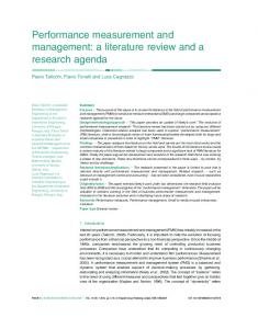
For example, we can represent performance data of Java interpreter activities like thread context switches, method table lookups, garbage collection, and bytecode instruction execution associated with dierent method functions in a Java application. We present results from a prototype implementation of our model for measuring the performance of interpreted Java applications and applets. Our prototype tool uses Paradyn's dynamic instrumentation [4] to dynamically insert and remove instrumentation from the Java virtual machine and Java method byte-codes as the byte-code is interpreted by the Java virtual machine. Our tool requires no modi cations to the Java virtual machine nor to the Java source nor class les prior to execution. The diculties in measuring the performance of interpreted codes is demonstrated by comparing an interpreted code's execution to a compiled code's execution. A compiled code is in a form that can be executed directly on a particular operating system/architecture platform. Performance tools for compiled code provide performance measures in terms of platform-speci c costs associated with executing the code; process time, number of page faults, and I/O blocking time are all examples of platform-speci c measures. In contrast, an interpreted code is in a form that can be executed by the interpreter virtual machine. The interpreter virtual machine is itself an application program that executes on some operating system/architecture platform. One obvious dierence between compiled and interpreted application execution is the extra layer of the interpreter program that, in part, determines the application's performance (see Figure 1). A performance tool for measuring the performance of an interpreted execution needs to measure the interaction between the Application layer (AP) and the InterpreterVM layer (VM). There are potentially two dierent program developers that would be interested in performance measurement of the interpreted execution: the virtual machine developer and the application program developer. Both want performance data described in terms of platform-speci c costs associated with executing parts of their program. However, each views the platform and the program as dierent layers of the interpreted execution. The VM developer sees the AP as input to the VM program that is run by the Platform layer (left side of the interpreted execution in Figure 1). The AP developer sees the Application layer as the program that is run on the VM (right side of the interpreted execution in Figure 1). For a VM developer, this means characterizing the virtual machine's Compiled Execution Application Platform (Os/Arch)

Interpreted Execution VM developer’s view: input application platform

Application

AP developer’s view: application

InterpreterVM platform

Platform (Os/Arch)

Fig. 1. Compiled application's execution vs. Interpreted application's execution. VM and AP developers view the interpreted execution dierently.

performance in terms of Platform layer costs of the VM program's execution of its input (AP)|for example, the amount of process time executing VM function invokeMethod while interpreting AP method foo. The application program developer wants performance data that measures the same interaction to be de ned in terms of VM-speci c costs associated with AP's execution; for example, the amount of method call context switch time in AP method foo. Another characteristic of an interpreted execution is that the application program has multiple execution forms. By multiple execution forms we mean that AP code is transformed into another form or other forms while it is executed. For example, a Java class is read in by the Java VM in .class le format. It is then transformed into an internal form that the Java VM executes. This diers from compiled code where the application binary is not modi ed as it executes. Our model characterizes AP's transformations as a measurable event in the code's execution, and we represent the relationship between dierent forms of an AP code object so that performance data measured for one form of the code object can be mapped back, to be viewed in previous forms of the object.

2 Performance Measurement Model We present a representational model for describing performance data from an interpreted execution that explicitly represents the interaction between the application program and the virtual machine. Our model addresses the problems of representing an interpreted execution and describing performance data from the interpreted execution in a language that both the virtual machine developer and the application program developer can understand.

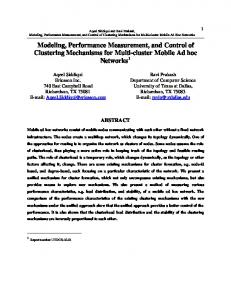
2.1 Representing an Interpreted Execution Our representation of an interpreted execution is based on Paradyn's representation of a program execution as a set of resource hierarchies. A resource is a physical or logical component of a program (a semaphore, a function, and a process are all examples of program resources). A resource hierarchy is a collection of hierarchically related program resources. For example, the Process resource hierarchy views the running program as a set of processes. It consists of a root node that represents all processes in the application, and some number of child resources|one for each process in the running program. Other examples of resource hierarchies are a Code hierarchy for the code view of the program, a Machine hierarchy for the set of machines on which the application is running, and a Synchronization hierarchy for the set of synchronization objects in the application. An application's execution might be represented as the following set of resource hierarchies: fProcess, Machine, Code, SyncObjg. An individual resource is represented by a path from its root node. For example, the function resource main is represented by the path /Code/main.C/main. Its path represents its relationship to other resources objects in the Code hierarchy.

Virtual Machine Machine cham grilled

Code

Process

main.c blah.c

pid 1 pid 2 pid 3

Application Program SyncObj msg tag 1 2

Code main foo foo blah

Threads tid 1 tid 2 tid3

SyncObj monitors mon1 mon2

Fig. 2. Example resource hierarchies for the virtual machine and the application program.

Since both the application program and the virtual machine can be viewed as executing programs, we can represent each of their executions as a set of resource hierarchies. For example, AP's execution might be represented by fCode, Thread, SyncObjg (right half of Figure 2), and the virtual machine's execution might be represented as fMachine, Process, Code, SyncObjg (left half of Figure 2). The resource hierarchies in this gure represent AP and VM's executions separately. However, there is an interaction between the execution of the two that must be represented. The relationship between the virtual machine and its input (AP) is that VM runs AP. We represent the VM runs AP relationship as an interaction between program resources of the two; code, process, and synchronization objects in the virtual machine interact with code, process, and synchronization objects in the application program during the interpreted execution. The interpreted execution is the union of AP and VM resource hierarchies. Figure 3 is an example of an interpreted execution represented by fMachine, Code, Process, SyncObj, APCode, APThreads, APSyncObjg. The application program's multiple execution forms are represented by a set of sets of resource hierarchies{one set for each of the forms that AP takes during its execution, and a set of mapping functions that map resources in one form to resources in another form of AP. For example, in a dynamically compiled Java application, method functions may be translated from byte-code form to native code form during execution. Initially we create one AP Code hierarchy for the byte-code form of AP. As run-time transformations occur, we create a new AP code hierarchy for the native form of AP objects, and create mapping functions that map resources in one form to resources in the other form.

VM runs AP Machine

Code

Process

SyncObj

APCode

cham grilled

main.c blah.c

pid 1 pid 2 pid 3

msg tag 1 2

main foo foo blah

APThreads tid 1 tid 2 tid3

APSyncObj monitors mon1 mon2

Fig. 3. Resource hierarchies representing the execution of VM runs AP.

2.2 Representing Points in an Interpreted Execution We can think of a program's execution as a series of events. Executing an instruction, waiting on a synchronization primitive, and accessing a memory page are examples of events. Any event in the program's execution can be represented as a subset of its active resources|those resources that are currently involved in the event. For example, if the event is \process 1 is executing code in function foo", then the resource /Code/main.C/foo and the resource /Process/pid 1 are both active when this activity is occurring. These single resource selections from a resource hierarchy are called constraints. The activity speci ed by the constraint is active when its constraint function is true.

De nition 1. A constraint is a single resource selection from a resource hierarchy. It represents a restriction of the hierarchy to some subset of its resources.

De nition 2. A constraint function, constrain(r), is a boolean function of resource r that is true when r is active. For example, constrain(/Process/pid 1) is true when process 1 is active (i.e. running). Constraint functions are resource-speci c; all constraint functions test whether their resource argument is active, but the type of test that is done depends on the type of the resource argument. The constraint function for a process resource will test whether the speci ed process is running. The constraint function for a function resource will test whether the program counter is in the function. Each resource hierarchy exports the constraint functions for the resources in its hierarchy. For example, Code.constrain(/Code/main.C) is the constraint function applied to the Code hierarchy resource main.C. Constraint functions can be combined with AND and OR to create boolean expressions containing constraints on more than one resource. By combining one constraint from each resource hierarchy with the AND operator, we represent dierent activities in the running program. This representation is called a focus.

De nition 3. A focus is a selection of resources (one from each resource hierarchy). It represents an activity in the running program. A focus is active when all of its resources are active (i.e., the AND of the constraint functions).

If the focus contains resources that are re ned on both VM and AP resource hierarchies, then it represents a speci c part of virtual machine's execution of the application program. For example, is a focus from Figure 3 that represents when VM's process 1 is executing function invokeMethod, and interpreting AP method foo. This activity is occurring when the corresponding constraint functions are all true.

2.3 Performance Data for Interpreted Execution To describe performance data that measure the interaction between the application program and the virtual machine, we provide a mechanism to selectively

constrain performance information to any part of the execution. There are two complementary (and occasionally overlapping) ways to do this: constraints are either implicitly speci ed by metric functions or explicitly speci ed by foci. A metric function is a time-varying function that measures some aspect of a program execution's performance. Metric functions consist of time or count functions combined with boolean expressions built from constraint functions and constraint operators. For example:

{ CPUtime = [ ]processTime/sec. The amount of process time per second. { methodCallTime = [Code.constrain(/Code/main.C/invokeMethod)] processTime/sec. The time spent in VM function invokeMethod. { io wait = [Code.constrain(/Code/libc.so/read) OR Code.constrain( /Code/libc.so/write)] wallTime/sec. The time spent reading or writing. The second way to constrain performance data is by specifying foci that represent restricted locations in the execution. Foci with both VM and AP resources represent an interaction between VM and AP. The focus represents the part of the execution when the virtual machine is fetching AP code object foo. This part of the execution is active when [Code.constrain( /Code/main.C/fetchCode) AND APCode.constrain( /APCode/foo.class/foo)] is true. If we combine metric functions with

this focus, we can represent performance data for the speci ed interaction. We represent performance data as metric-focus pairs. The AND operator is used to combine a metric with a focus. The following are some example metric{ focus pairs (we only show those components of the focus that are re ned beyond a hierarchy root node): 1. CPUtime, : [ ] processTime/sec AND [APCode.constrain(/APCode/foo.class/foo)] 2. CPUtime, : [ ] processTime/sec AND [Code.constrain(/Code/main.C/invokeMethod) AND APCode.constrain(/APCode/foo.class/foo)] 3. methodCallTime, : [Code.constrain(/Code/main.C/invokeMethod)] processTime/sec AND [APCode.constrain(/APCode/foo.class/foo)]

Example 1 measures the amount of process time spent in AP function foo. The performance measurements in examples 2 and 3 are identical|both measure the amount of process time spent in VM function invokeMethod while interpreting AP function foo. However, example 2 is represented in a form that is more useful to a VM developer and example 3 is represented in a form that is more useful to an AP developer. Example 3 uses an VM-speci c metric. VM-speci c metric functions measure activities that are speci c to a particular virtual machine. They are designed to present performance data to an AP developer who may have little or no knowledge of the virtual machine; they encode knowledge of the virtual machine in a representation that is closer to the semantics of the application language. Thus, an AP developer can measure VM costs associated with the execution of their program without having to know the details of the

implementation of the VM; the methodCallTime metric encodes information about the VM function invokeMethod that is used to compute its value. A nal issue is representing performance data for foci with application program resources. An AP object may currently be in one form, while its performance data should be viewable in any of its forms. To do this, AP mapping functions are used to map performance data that is measured in one form of an AP object to a logical view of the same object in any of its other forms.

3 Measuring Interpreted Java applications We present a tool for measuring the performance of interpreted Java applications and applets running on Sun's version 1.0.2 of the Java VM [6]. The tool is an implementation of our model for representing performance data from an interpreted execution. The Java VM is an abstract stack-based processor architecture. A Java program consists of a set of classes, each compiled into its own .class le. Each method function is compiled into byte-code instructions that the VM executes. To measure the performance of an interpreted Java application or applet, our performance tool (1) discovers Java program resources as they are loaded by the VM, (2) generates and inserts SPARC instrumentation code into Java VM routines, and (3) generates and inserts Java byte-code instrumentation into Java methods and triggers the Java VM to execute the instrumentation code. Since the Java VM performs delayed loading of class les, new classes can be loaded at any point during the execution. We insert instrumentation code in the VM that noti es our tool when a new .class le is loaded. We parse the VM's internal form of the class to create application program code resources for the class. At this point, instrumentation requests can be made for the class by specifying metric{focus pairs containing the class's resources. We use dynamic instrumentation [4] to insert and delete instrumentation into Java method code and Java VM code at any point in the execution. Dynamic instrumentation is a technique where instrumentation code is generated in the heap, a branch instruction is inserted from the function's instrumentation point to the instrumentation code, and the function's instructions that were replaced by the branch are relocated to the heap and executed before or after the instrumentation code. Because the SPARC instruction set has instructions to save and restore stack frames, the instrumentation code and the relocated instructions can execute in their own stack frames. Thus instrumentation code will not destroy the values in the function's stack frame. Using this technique to instrument Java methods is complicated by the fact that a method's byte-code instructions push and pop operands from their own operand stack. Java instrumentation code should use its own operand stack and have its own execution stack frame. The Java instruction set does not contain instructions to explicitly save and restore execution stack frames or to create new operand stacks. Our solution uses a technique called transformational instrumentation. This technique forces the Java VM to create a new operand stack

and execution stack frame for our instrumentation code. The following are the transformational instrumentation steps:

1. The rst time an instrumentation request is made for a method, relocate the method byte-code to the heap and expand its size by adding nop byte-code instructions around each instrumentation point. The nop instructions will be replaced with branches to instrumentation code. 2. Get the VM to execute the relocated method byte-code by replacing the rst bytes in the original method with a goto w byte-code instruction that branches to the relocated method. Since the goto w instruction is inserted after the VM has veri ed that this method byte-code is legal, the VM will execute this instruction even though it branches outside the original method function. 3. Generate instrumentation code in the heap. We generate SPARC instrumentation code in the heap, and use Java's native methods facility to call our instrumentation code from the Java method byte-code. 4. Insert method call byte-code instructions in the relocated method to call the native method function that will execute the instrumentation code. This will implicitly cause the VM to create a new execution stack frame and value stack for the instrumentation code.

4 Results We present results from running a Java application with our performance tool. The application is a CPU scheduling simulator that consists of eleven Java classes and approximately 1200 lines of Java code. Currently, we can represent performance data in terms of VM program resources, AP code resources, and the combination of VM and AP program resources using both foci and VM-speci c metrics to describe the interaction. Figure 4 shows the resource hierarchies from the interpreted execution, including the separate VM and AP code hierarchies. We began by looking at the overall CPU utilization of the program (about 98%). We next tried to account for the part of the CPU time due to method call context switching and object creation in the Java VM. To measure these, we created two VM-speci c metrics|MethodCall CS measures the time for the Java VM to perform a method call context-switch, and obj create measures the time for the Java VM to create a new object. Both are a result of the VM interpreting certain byte-code instructions in the AP. We measured these values for the Whole Program focus (no constraints). As a result, we found that a

Fig. 4. Resource Hierarchies from the interpreted execution.

Fig. 5. Time Histogram showing CPU utilization, object creation time, and method call context switching time. This graph shows that method call context switching time plus object creation time account for  35% of the total CPU time. large portion ( 35%) of the total CPU time is spent handling method context switching and object creation (Figure 5)2 . Because of these results, we rst tried to reduce the method call context switching time by in-lining method functions. Figure 6 shows the method functions that are accounting for the most CPU time and the largest number of method function calls. We found that the nextInterrupt() and isBusy() methods of the Device class were being called often, and were accounting for a relatively large amount of total CPU time. By examining the code we found that the Sim.now() method was also called frequently. These three methods return the value of a private data member, and thus are good candidates for in-lining. After changing the code to in-line calls to these three method functions, the total number of method calls decreased by 31% and the total execution time decreased by 12% (second row in Table 1). We next tried to reduce the object creation time. We examined the CPU time for the new version of the AP code, and found that the Sim, Device, Job, and StringBuffer classes accounted for most of the CPU time. The time spent in StringBuffer methods is due to a large number of calls to the append and constructor methods made from the Sim and Device classes. We were able to reduce the number of StringBuffer and String objects created by removing strings that were created but never used, and by creating static data members for parts of strings that were recreated multiple times (in Device.stop() and Device.start()). With these changes we are able to reduce the total execution time by 70% (fourth row in Table 1). 2

With CPU enabled for every Java class, about 45% is due to executing Java code, 5% to method call context switching, and 40{45% to instrumentation overhead.

Fig. 6. AP classes and methods that account for the largest % CPU (left) and that are called the most frequently (right). The rst column lists the focus, and the second column lists the metric value for the focus. Table 1. Performance results from dierent versions of the application.

Optimization

Number of Number of Total Execution Method Calls Object Creates Time (in seconds) Original Version 13,373,200 465,140 389.29 Method in-lining 9,213,400 (31% less) 465,140 343.99 (-12% change) Fewer Obj. Creates 9,727,800 (27% less) 17,350 (96% less) 234.13 (-40% change) Both Changes 5,568,100 (58% less) 17,350 113.60 (-70% change)

In this example, our tool provided performance data that is dicult to obtain with other performance tools. Our tool provided performance data that described expensive interactions between the Java VM and the Java application, and accounted for these costs in terms of AP resources. With this data, we were easily able to determine what changes to make to the Java application to improve its performance.

5 Related Work There are many general purpose program performance measurement tools [3, 5, 7, 4] that can be used to measure the performance of the virtual machine. However, these are unable to present performance data in terms of the application program or in terms of the interaction between VM and AP. There are some performance tools that provide performance data in terms of AP's execution [1, 2]. These tools provide performance data in terms of Java application code. However, they do not represent performance data in terms of the Java VM's execution or in terms of the interaction between the VM and the Java application. If the time values provided by these tools include Java VM method call, object creation, garbage collection, thread context switching, or class le loading activities in the VM, then performance data that explicitly represents

this interaction between the Java VM and the Java application's execution will help an application developer determine how to tune his or her application.

6 Conclusion and Future Work This paper describes a new approach to performance measurement of interpreted executions that explicitly models the interaction between the interpreter program and the interpreted application program so that performance data can be associated with any part of the execution. Performance data is represented in terms that either an application program developer or an interpreter developer can understand. Currently, we are working to expand our prototype to include a larger set of VM-speci c metrics, AP thread and synchronization resource hierarchies, and support for mapping performance data between dierent views of AP code objects. With support for AP thread and synchronization resources our tool can provide performance data for multi-threaded Java applications.

7 Acknowledgments Thanks to Marvin Solomon for providing the CPU simulator Java application. This work is supported in part by DARPA contract N66001-97-C-8532, NSF grant CDA-9623632, and Department of Energy Grant DE-FG02-93ER25176. The U.S. Government is authorized to reproduce and distribute reprints for Governmental purposes notwithstanding any copyright notation thereon.

References 1. Intuitive Systems. Optimize It. http://www.optimizeit.com/. 2. KL Group. JProbe. http://www.klg.com/jprobe/. 3. A. Malony, B. Mohr, P. Beckman, D. Gannon, S. Yang, and F. Bodin. Performance Analysis of pC++: A Portable Data-Parallel Programming System for Scalable Parallel Computers. Proceedings of the 8th International Parallel Processing Symposium (IPPS), Cancun, Mexico, pages 75{85, April 1994. 4. B. P. Miller, M. D. Callaghan, J. M. Cargille, J. K. Hollingsworth, R. B. Irvin, K. L. Karavanic, K. Kunchithapadam, and T. Newhall. The Paradyn Parallel Performance Measurement Tools. IEEE Computer 28, 11, November 1995. 5. D. A. Reed, R. A. Aydt, R. J. Noe, P. C. Roth, K. A. Shields, B. W. Schwartz, and L. F. Tavera. Scalable Performance Analysis: The Pablo Performance Anlysis Environment. Proceedings of the Scalable Parallel Libraries Conference, pages 104{ 113. IEEE Computer Society, 1993. 6. Sun Microsystems Computer Corporation. The Java Virtual Machine Speci cation, August 21 1995. 7. J. C. Yan. Performance Tuning with AIMS { An Automated Instrumentation and Monitoring System for Multicomputers. 27th Hawaii International Conference on System Sciences, Wailea, Hawaii, pages 625{633, January 1994. This article was processed using the LATEX macro package with LLNCS style