ISA TRANSACTIONS® ISA Transactions 43 共2004兲 133–151
Performance index for quality response of dynamical systems Manuel A. Duarte-Mermoud,* Rodrigo A. Prieto Department of Electrical Engineering, University of Chile, Casilla 412-3, Santiago, Chile
共Received 2 January 2002; accepted 9 June 2003兲
Abstract The use of performance indices to measure the quality response of dynamical systems is studied in this paper. A definition of a general performance index is proposed which is easy to compute, easy to interpret, and flexible enough to account for different cases commonly presented in practice. The index is tested over several dynamical responses obtained from different systems obtaining good results, in the sense that it is able to rank the behaviors from best to worse, compared with a pattern response. © 2004 ISA—The Instrumentation, Systems, and Automation Society. Keywords: Performance index; Quality response; Transient response
1. Introduction Nowadays the majority of industrial plants work under control, where not only stability but also performance is of great importance. Measuring the quality of a system response is a tough problem. Over the years, several quality performance indices have been proposed in the control literature for measuring the response quality of a controlled system. The first indices were proposed in the early 1950s and correspond to the very well known integral of the absolute magnitude of the error 共IAE兲, integral of the time multiplied by the absolute magnitude of the error 共ITAE兲, integral of the square of the error 共ISE兲, and integral of the time multiplied by the square of the error 共ITSE兲 关1–5兴, which are based on the analysis of the control error signal. More recently, several transient improvement methods have been studied and measures of the response quality have been proposed in the context of adaptive controllers 关6 –10兴. One *Author to whom all correspondence should be addressed. E-mail address:
[email protected]
of them proposes a method of bounding the output for a certain arbitrary instant of time 关6兴, whereas others propose as a measure the norm L ⬁ 关7–9兴, the norm L 2 关9兴 or the square or integral of square 关10兴 of the control error. We have to recognize the difficulty of finding one simple index able to discriminate the best response among a series of responses coming from different dynamical systems. One of the most serious difficulties is to decide what characteristics of the system response are important to take into account and how they have to be weighted 共if they are not considered totally equal兲. A general and versatile index is proposed in this paper, based on several characteristics considered important in a system response. These characteristics can be suitably weighted to emphasize their importance in the general index 关11,12兴. After some general concepts introduced in Section 2, the response characteristics to be considered in this study are described in Section 3. In Section 4 the definition of a general and flexible performance index is proposed. This index is tested for several dynamical systems in Section 4,
0019-0578/2004/$ - see front matter © 2004 ISA—The Instrumentation, Systems, and Automation Society.
134
Manuel A. Duarte-Mermoud, Rodrigo A. Prieto / ISA Transactions 43 (2004) 133–151
where analysis and comparisons of the index are performed. Finally, some conclusions are drawn in Section 5. 2. General concepts The concept of desired behavior for a controlled system immediately states a goal for the dynamical system under study. We will call this desired behavior pattern response and the actual behavior of the system to be analyzed is called system response. In all the definitions introduced in this paper we will use the subindex p when referring to the pattern response and the subindex c when referring to system response. It is also important to define the control error signal as the difference between the reference and the system response, which will give us an idea as to how far the system response is from the desired value at every instant of time,
e 共 t 兲 ⫽r 共 t 兲 ⫺y 共 t 兲 .
共1兲
For notation purposes we will denote y c( t ) as the response of the system under analysis and y p ( t ) as the pattern response. Given the response of a dynamical system under control it is pertinent to ask what characteristics of that response are important for the designer. In what follows we define a set of characteristics belonging to the system response. This set is only a representative set of characteristics and many others could be added to enrich the final performance index. Some of these characteristics are associated to the steady-state regime and some others to the transient period. Only temporal characteristics are considered in this study though frequency characteristics could have also been considered, using the same methodology stated in the paper. The definition of the pattern response for a given process is not straightforward. The same ideas and guidelines used, for example, in the model reference adaptive control 共MRAC兲 when the reference model has to be defined can be employed here. On the other hand, a control engineer knows pretty well what is a good response for his process, so the problem of identifying the pattern response for a given process is not an issue, the main issue for them is how to get it. It is a generalized practice for control purposes around an operation point to use first- or second-order models of the plant and eventually a delay between the
Fig. 1. Typical form of index of type 1.
input and the output. It is possible then to choose as a pattern response, for example, the response of a second-order plant under a unit step input with the poles conveniently located to obtain a reasonable overshoot 共or none兲 and a suitable settling time, to name only a few characteristics. That could be a good starting point to define a suitable pattern response. Since our objective is to numerically determine how close is the system response with respect to the pattern response, we proceed to define a characteristic index 共ci兲 associated to each characteristic of interest defined for the system response. This index, denoted as I with a proper subindex, will give the semblance of the characteristic exhibited by the system response with respect to that present in the pattern response. Each ci is built in such a fashion that introducing the necessary information for the pattern and system response, the computation provides a normalized value in the interval 关0,1兴. A value close to 1 will indicate a good correspondence between the characteristic of the system response as compared with that of the pattern response. On the contrary, a value near zero indicates that the characteristic of the system response has little to do with that of the pattern response. To guarantee its variation between 0 and 1, a piecewise function is defined according to specific criteria for each characteristic under study. There are usual cases to compute the ci as a function of a system response characteristic ( c c ) and the corresponding pattern response characteristic ( c p ) . We classify these indices in three types. 2.1. Type-1 index This index is built according to the following criteria 共see Fig. 1兲: • The index is zero if c c is outside the interval 关 0,c pm兴 , meaning that any value of c c out-
Manuel A. Duarte-Mermoud, Rodrigo A. Prieto / ISA Transactions 43 (2004) 133–151
135
side the limits of the interval is considered too far from the right value and therefore not good. • The index is 1 if and only if c c ⫽c p . • Finally, if c c is inside the interval 关 0,c pm兴 , the index value decays in some way from 1 to c pm and from 1 to 0.
c pm is a maximum value defined by the designer and typical value of c pm is taken as 2c p . The decay used could be exponential 共if a strong decay is needed兲 or polynomial. Using an exponent of 0.02 in a type-1 index with exponential decay means a strong penalization of the characteristic when even small deviations are present in the actual response with respect to the desired one. This can be concluded from the sharpness of the curve around the value one shown in Fig. 1. Let us consider, e.g., the index defined by Eq. 共2兲 and suppose that the deviation between both characteristics is only 1%, then the index value decreases to the value 0.862 共i.e., diminishes in about 13.8% with respect to the ideal case兲. If instead the deviation is 5% the index takes the value 0.316, diminishing the index value in 68.4%. Finally, if the deviation is 10% the index is only 0.165, a very small value, penalizing a deviation of 10% in about 83.5% with respect to the ideal case. On the other hand, if this penalization is considered excessive the exponent should be increased and a value of 0.08 could then be used. In that case a deviation of 1% makes the index go to a value of 0.999, a deviation of 5% yields an index value of 0.781, and a deviation of 10% gives an index value of 0.513, which means that the penalization effect is rather weak if compared with the case of exponent 0.02. The same discussion applies to the case when polynomial instead of exponential decay function is used. The exponent 2 is used when a rather weak penalization is called for whereas exponent 4 is used when a stronger decay is needed. Another important fact in this case is that the flatness of the index around the value 1 is evident, penalizing weakly rather large deviations around the ideal value 共see, for example, Fig. 10兲.
Fig. 2. Typical variation of a type-2 index.
• If c c ⭐c p , i.e., the characteristic of the system response is less than that of the pattern response, this is considered good and the index takes the value 1. • If c c is inside the interval ( c p , c pm] , the index value decays in some way to zero. This decay could be exponential or polynomial, according to the designer objectives. 2.3. Type-3 index The index is built according to certain criteria giving a variation shown in Fig. 3: • If c c is inside the interval 关 ( 1⫺ ) c p , ( 1 ⫹ ) c p 兴 this situation is considered good and the index takes the value 1. • If c c is outside the interval 关 ( 1⫺ ) c p , ( 1 ⫹ ) c p 兴 , the index value decays in some way to zero and to c pm . This decay could be exponential or polynomial, according to the designer objectives. Though the type-1 index could be considered as a type-3 index with ⫽0, the two cases were separated to make evident the dead zone in the case of the type-3 index.
2.2. Type-2 index The index is built according to certain criteria giving a variation shown in Fig. 2:
Fig. 3. Typical variation of a type-3 index.
136
Manuel A. Duarte-Mermoud, Rodrigo A. Prieto / ISA Transactions 43 (2004) 133–151
3. Response characteristics and characteristic indices In what follows we will define a set of response characteristics to be considered in the study and we will derive the corresponding ci. 3.1. Steady-state value (ssv) The steady state value 共ssv兲 is the value reached by the system response as time goes to infinity, when a constant input is applied. When ssv is compared with the final value of the reference 共set point兲 the steady-state error arises. For computation purposes the last sixth part of the system error signal is considered and then it is verified that there is no point beyond a given tolerance around the mean value of the whole signal. If so, the mean value of the whole signal is considered as the bias of the error signal and the mean value of the last sixth part of the error signal as the ssv of the error signal. In case the condition is not satisfied the tolerance is increased until the condition is met. The ci associated to the ssv, denoted as I ssv , tells us how close is the ssv of the system response under study ( ssvc ) as compared with that of the pattern response ( ssvp ) . The necessary information to compute this index is the knowledge ssvc and ssvp . This index is of type 1 and it is computed by Eq. 共2兲, using the criteria given in Section 2.1,
I ssv⫽
冦
0 if ssvc 苸 b 0,2•ssvp c 0.02•ssvc 1⫺exp if ssvc 苸 关 0,ssvp 兲 ssvc ⫺ssvp 1 if ssvc ⫽ssvp 0.02• 共 2•ssvp ⫺ssvc 兲 1⫺exp ssvp ⫺ssvc if ssvc 苸 共 ssvp ,2•ssvp 兴 . 共2兲
冉 冉
冊
冊
The plot of this index is similar to that shown in Fig. 1, with c p ⫽ssvp and c c ⫽ssvc . 3.2. Settling time (ts) Conceptually the settling time is the time at which the response enters 共and does not come outside again兲 inside a band around the steady-state value. A typical band is ⫾5%, it being also pos-
Fig. 4. Bands around the ssv to define ts.
sible to define other bands such as ⫾0.5%, ⫾1%, ⫾2%, ⫾10%, ⫾20%, and ⫾50%. In Fig. 4, some of these bands are shown. The necessary information to compute ts for a certain band is the time variable, the response value at the very instant of time and the lower and upper limit of the selected band. The corresponding characteristic index ( I ts) gives thesimilarity between the ts of the system response ( tsc ) and the ts of the pattern response ( tsp ) . In this study we consider the bands ⫾5%, ⫾20%, and ⫾50%, it being possible to change some of them or to choose others if the circumstances advise it. The necessary information for computing the index is tsc , tsp , and the final time considered for the study t f . This index is of type 2 and is based on the criteria explained in Section 2.2. The function to compute the index is given by Eq. 共3兲, which has a plot like that of Fig. 2 with c p ⫽tsp and c cf⫽t f ,
再冉
1 if tsc 苸 b 0,tsp c
I ts⫽
兩 t f ⫺tsc 兩 兩 t f ⫺tsp 兩
冊
3
if tsc 苸 共 tsp ,t f 兴 .
共3兲
3.3. IAE, ITAE, ISE, and ITSE indices From the error signal defined in Eq. 共1兲 it is possible to compute the very well-known IAE, ITAE, ISE, and ITSE indices, defined as integral expressions related to the control error 关3兴 as follows. • IAE index: This index corresponds to the integral of the error absolute value as shown in Eq. 共4兲,
Manuel A. Duarte-Mermoud, Rodrigo A. Prieto / ISA Transactions 43 (2004) 133–151
IAE⫽
冕 兩e共 t 兲兩dt. ⬁
0
137
共4兲
The IAE reflexes the cumulative error, i.e., how far the response is with respect to the applied reference. • ITAE index: This index represents the integral of the error absolute value but weighted by time as shown in Eq. 共5兲,
ITAE⫽
冕 t兩e共 t 兲兩dt. ⬁
0
共5兲
It gives less importance to initial errors, whereas the present errors are much more considered. • ISE index: This index is defined as the integral of the square error, as shown in Eq. 共6兲,
ISE⫽
冕 e 共 t 兲dt. ⬁
2
0
共6兲
The index is associated to the error energy, giving more importance to larger errors and less importance to small errors. • ITSE index: This index is similar to the previous one but it is weighted by time 关see Eq. 共7兲兴,
ITSE⫽
冕 te 共 t 兲dt. ⬁
2
0
共7兲
This index gives very little importance to initial errors as compared with most recent ones. Based on these indices we define the corresponding characteristic indices I IAE , I ITAE , I ISE , and I ITSE . They are evaluated from the IAE, ITAE, ISE, and ITSE indices corresponding to the system response 关using the error e c ( t ) ⫽r ( t ) ⫺y c ( t ) ] and the pattern response 关using the error e p ( t ) ⫽r ( t ) ⫺y p ( t ) ] . These indices are of type 2 and following the general criteria of Section 2.2 we define it as
I⫽
再
1 if c c ⭐c p exp关 ⫺0.5• 共 c c ⫺c p 兲兴 if c c ⬎c p ,
共8兲
where c c is the characteristic associated to the system response ( IAEc , ITAEc , ISEc , ITSEc ) and c p is the characteristic associated to the pattern response ( IAEp , ITAEp , ISEp , ITSEp ) . The form of the index is similar to Fig. 2.
Fig. 5. Description of areas over and under the ssv.
3.4. Areas around the ssv (ap, an) Given the ssv of the system response one interesting characteristic is the cumulative area over the ssv 共denoted as ap兲 and under the ssv 共denoted as an兲, as shown in Fig. 5. The addition of areas api and ani give the total areas over 共ap兲 and under 共an兲 the ssv as indicated in Eqs. 共9兲 and 共10兲, respectively,
a p⫽ 兺 a pi,
共9兲
a n⫽ 兺 a ni.
共10兲
i⫽1
i⫽1
To quantify the similarity of the area over the ssv of the system response ( apc ) with respect the area over the ssv of the pattern response ( app ) we define the corresponding ci ( I ap) . To compute this characteristic index the following information is needed:
app : area over the ssv of pattern response; apc : area over the ssv of system response; ssvp : steady-state value of pattern response; ts5 p : settling time of pattern response 共⫾5% band兲. The total area cumulated was considered until time ts rather than final time t f . Thus we define the concept of maximum tolerance of pattern response ( tmap ) as follows:
tmap ⫽ssvp •t s5 p .
共11兲
Case 1. We consider that any value of app is negligible if it does not exceed 1% of tmap . The following three criteria are then introduced for the case when app 苸 关 0,0.01•tmap 兴 关see Eq. 共12兲兴.
138
Manuel A. Duarte-Mermoud, Rodrigo A. Prieto / ISA Transactions 43 (2004) 133–151
Fig. 6. 共a兲 ci associated to the area over the ssv (I ap), for the case app 苸 关 0,0.01•tmap 兴 . 共b兲 ci associated to the area over the ssv (I ap), for the case app ⬎0.01•tmap .
• If apc 苸 关 0,0.01•tmap 兴 the index will take the value 1, since the characteristic of the system response and pattern response belong to the same interval, considered both negligible. • If apc ⬎tmap the index will be zero, since a value of apc greater than the maximum area tolerance is considered excessive. • If apc 苸 关 0.01•tmap ,tmap 兴 , then the function used to compute the index is of exponential type with argument 0.08, giving an initially strong decay and then moderate from 1 to 0 关see Fig. 6共a兲兴. Case 2. If app ⬎0.01•tmap it is considered a not negligible value applying the following three criteria 关see Eq. 共12兲兴. • If apc ⫽app the index is unity. • If apc is outside the interval 关 0,2•app 兴 the index is zero since the characteristic of the system response is at least twice the pattern response, which is considered unacceptable. • Finally, if apc belongs to 关 0,app ) 艛 ( app , 2•app 兴 , the index is computed by means of a cubic function whose argument is the difference between unity and 兩 apc ⫺app 兩 with respect to app . Thus we assure that the index is greater than 0.5 only when the characteristic of the system response is around the ⫾25% of the characteristic of the pattern response 关see Fig. 6共b兲兴. Considering the two previous cases the function for I ap is then given by Eq. 共12兲 and plotted in Figs. 6共a兲 and 6共b兲,
1 if app 苸 关 0,0.01•tmap 兴 and apc 苸 关 0,0.01•tmap 兴 0 if app 苸 关 0,0.01•tmap 兴 and apc 苸 关 0,tmap 兴 , 0.08"共 apc ⫺tmap 兲 1⫺exp apc if app 苸 关 0,0.01•tmap 兴 I ap⫽ and apc 苸 共 0.01•tmap ,tmap 兴 1 if app ⬎0.01•tmap and apc ⫽app 0 if app ⬎0.01•tmap and apc 苸 关 0,2"app 兴 兩 app ⫺apc 兩 3 1⫺ if app ⬎0.01•tmap app and apc 苸 关 0,app 兲 艛 共 app ,2•app ]. 共12兲
¦
冉
冉
冊
冊
To quantify the similarity of the area under the ssv of the system response ( anc ) as compared with the area under the ssv of the pattern response ( anp ) we define the corresponding ci denoted as I an . To define this index we use the same procedure already explained for the areas over the ssv. In this case we need information regarding
anp : area under the ssv of pattern response; anc : area under the ssv of system response; ssvp : steady-state value of pattern response; ts5 p : settling time of pattern response ( ⫾5% band兲. Eq. 共12兲 is used here to compute the index I an , changing app by anp and apc by anc .
Manuel A. Duarte-Mermoud, Rodrigo A. Prieto / ISA Transactions 43 (2004) 133–151
3.5. Area deviation around the ssv (dap, dan) This characteristic allows us to visualize the area distribution in 关 °/1兴 , around the ssv of the system response. The corresponding index is computed based on the information obtained in the previous section by calculating
aT⫽ap⫹an, dap⫽
ap , aT
an dan⫽ , aT
共13兲 共14兲 共15兲
where aT is the total area around the ssv, dap is the deviation area over the ssv of the system response in 关 °/1兴 , and dan is the deviation area under the ssv in 关 °/1兴 . The index I da estimates how close the percentage of area is over and under the ssv of the system response as compared with those of the pattern response. To assure its existence it is first verified that aT⫽0. The necessary information to compute this index is app , anp , aTp ⫽app ⫹anp , apc , anc , and aTc ⫽apc ⫹anc , from which Eqs. 共16兲–共19兲 are computed,
app dapp ⫽ , aTp
共16兲
apc , aTc
共17兲
danp ⫽
anp , aTp
共18兲
danc ⫽
anc . aTc
共19兲
dapc ⫽
Since the treatment for the case of area deviation over and under the ssv is similar we will make it in a unified way. In that sense we will define a generic pair dac and dap as follows:
再
共 dapc ,dapp 兲 共 dac ,dap 兲 ⫽ 共 dan ,dan 兲 . c p
共20兲
The index is defined using the following criteria:
139
• If dap ⫽0, the form of the function used is shown in Fig. 7共a兲, being a linear argument to the fourth power giving a unilateral decaying to zero. • If dap ⫽1, the function used is the same as before but the decaying is now from the value 1, as shown in Fig. 7共b兲. • If dap 苸 ( 0,1) , the computation procedure analyzes the cases when dap 苸 ( 0,0.5 兴 or dap 苸 ( 0.5,1 ) , applying the same function as before but with saturation of the index value in the nearest side 关see Figs. 7共c兲 and 共d兲兴. Based on the previous criteria the following function is built to give the ci I da associated to the area deviation 共over and under the ssv兲:
共 1⫺dac 兲 4 if dap ⫽0 共 dac 兲 4 if dap ⫽1
I da⫽
¦
冉
冉
1⫹
共 dac ⫺dap 兲 共 1⫺dap 兲
if dap 苸 共 0,0.5兴
and dac ⬍dap 1⫺
共 dac ⫺dap 兲 共 1⫺dap 兲
冉 冊 dac dap
冉
冊
4
冊
4
if dap 苸 共 0,0.5兴
and dac ⭓dap 4
if dap 苸 共 0.5,1兲 and dac ⬍dap
1⫺
共 dac ⫺dap 兲 dap
冊
4
if dap 苸 共 0.5,1兲
and dac ⭓dap . 共21兲
Figs. 7共a兲–7共d兲 show the behavior of the index.
3.6. Slope at the inflection point (s) When a step input is applied to a dynamical system the response is either in the same direction of the applied stimulus or in the opposite direction. When a positive step is applied and the response is in the positive direction, the slope of the response
140
Manuel A. Duarte-Mermoud, Rodrigo A. Prieto / ISA Transactions 43 (2004) 133–151
Fig. 7. 共a兲 ci associated to the area deviation (I da), for the case dap ⫽0. 共b兲 ci associated to the area deviation (I da), for the case dap ⫽1. 共c兲 ci associated to the area deviation (I da), for the case dap 苸(0,0.5 兴 . 共d兲 ci associated to the area deviation (I da), for the case dap 苸(0.5,1).
at the inflection point gives an idea of the reaction time. That is to say for two different systems the one with bigger slope is the one whose response is more rapid. To evaluate this characteristic it is necessary to compute the response first and second derivative. The procedure utilized here consists of determining, by means of cubic spline interpolation, the time at which the second derivative is zero 共inflection point兲. Then at that point the first derivative is evaluated 共slope response兲. Furthermore, the tangent is built as to have an estimation of the plant delay. In Fig. 8 it is shown a numerical example. The characteristic index ( I s ) associated to this characteristic quantify how close is the reaction time of the system response ( s c ) as compared with the reaction time of the pattern response ( s p ) . The information needed to compute this ci is s p and s c . To evaluate the similarity degree between both slopes we work with the corresponding angles. We define
␣ p : Angle associated to the pattern response at the inflection point 关see Eq. 共22兲兴. ␣ c : Angle associated to the system response at the inflection point 关see Eq. 共23兲兴.
Fig. 8. Details of the tangent at the inflection point 共0.206, 0.737兲.
Manuel A. Duarte-Mermoud, Rodrigo A. Prieto / ISA Transactions 43 (2004) 133–151
141
Fig. 11. Identification of overshoots and undershoots for a general response.
Fig. 9. Upper and lower limits for ␣ c .
␣ p ⫽arctan共 s p 兲 ,
共22兲
␣ c ⫽arctan共 s c 兲 .
共23兲
The maximum upper limit allowed for s c will be 2s p , i.e., the angle ␣ 2p given by Eq. 共24兲. The lower limit denoted by angle ␥ is determined as follows. First we define the auxiliary angle  which is computed as the difference between ␣ 2p and the pattern angle 关see Eq. 共25兲兴. Then the angle ␥ is computed as the difference between the pattern angle ␣ p and the auxiliary angle  关see Eq. 共26兲兴. Thus we get a symmetry of the interval with respect to the pattern characteristic,
be 关 ␥ , ␣ 2p 兴 , as shown in Fig. 9. Since this is not a typical index of type 1, 2, or 3 we will explain the criteria used in this case to build the index I s .
␣ 2p ⫽arctan共 2•s p 兲 ,
共24兲
• If ␣ c does not belong to interval 关 ␥ , ␣ 2 p 兴 , then the slope of the system response is considered to far from the pattern one and the index is set to zero. • On the contrary, if ␣ c 苸 关 ␥ , ␣ 2p 兴 , then the index is computed as the difference between 1 and a quadratic function whose argument is the quotient depending if ␣ c 苸 关 ␥ , ␣ p ) , or if ␣ c 苸 ( ␣ p , ␣ 2p 兴 , as shown in Eq. 共27兲.
 ⫽ ␣ 2p ⫺ ␣ p ,
共25兲
The general form of the index I s is plotted in Fig. 10.
␥ ⫽ ␣ p ⫺  ⫽2• ␣ p ⫺ ␣ 2p .
共26兲
Then the characteristics to be considered are ␣ c and ␣ p , whereas the variation interval for ␣ c will
I s⫽
冦
0 if ␣ c 苸 关 ␥ , ␣ 2p 兴
冉
冊
␣ p⫺ ␣ c 2 if ␣ c 苸 关 ␥ , ␣ p 兲 ␣ p⫺ ␥ 1 if ␣ c ⫽ ␣ p ␣ c⫺ ␣ p 2 1⫺ if ␣ c 苸 共 ␣ p , ␣ 2p 兴 . ␣ 2p ⫺ ␣ p 共27兲 1⫺
冉
冊
3.7. Sum of peaks, overshoot, and undershoot (spk, sov, sun)
Fig. 10. ci associated to the slope of the system response Is .
The sum of the overshoots and undershoots 共spk兲 of a system responsegive us an idea of the difficulty encountered by the system to reach the ssv. Similarly the separate summation of overshoots 共sov兲 and the summation of undershoots 共sun兲, are also considered since they give information that cannot be concluded from spk.
142
Manuel A. Duarte-Mermoud, Rodrigo A. Prieto / ISA Transactions 43 (2004) 133–151
Fig. 12. 共a兲 ci associated to the sum of overshoots and undershoots (I spk), for the case spkp ⫽0. 共b兲 ci associated to the sum of overshoots and undershoots (I spk), for the case spkp ⫽0.
Let us suppose that the response has n overshoots and m undershoots. All the overshoots and undershoots are measured considering a band of ⫾5% around the ssv. Then we can write 共see Fig. 11兲 n
m
j⫽1
k⫽1
spk⫽ 兺 兩 y 共 t j 兲 ⫺ssv兩 ⫹ 兺 兩 y 共 t k 兲 ⫺ssv兩 , 共28兲 n
sov⫽ 兺 兩 y 共 t j 兲 ⫺ssv兩 , j⫽1
共29a兲
m
sun⫽ 兺 兩 y 共 t k 兲 ⫺ssv兩 . k⫽1
共29b兲
The corresponding ci, denoted as I spk , indicates the degree of similarity between the distance from the ssv of the system response as compared with the pattern response. To compute the index the following information is needed:
spkp : spkc : ssvp :
summation of overshoots and undershoots for the pattern response; summation of overshoots and undershoots for the system response; steady state value of pattern response.
In building this index we distinguish two cases. Case 1. If spkp ⫽0, we will consider the following three criteria: • The index is set to zero if spkc does not exceed the 5% of the ssv of the pattern
response, since the difference is considered negligible. • On the other hand, if spkc exceed the 50% of the pattern response ssv, it is considered unacceptable and the index is set to zero. • On the contrary, if spkc is less than 50% but greater than the 5% of the pattern response ssv, the index is computed using an exponential of argument 0.08. This provides a strong initial decaying until a value 0.5 of the index, then the decaying continues smoothly until zero 关see Fig. 12共a兲兴. Case 2. If spkp ⫽0, its value will be greater than the 5% of ssvp , the following three criteria are used to compute the index. • A value of spkc greater than twice spkp is considered unacceptable and therefore the index is set to zero. • The index will have a value unity if spkp ⫽spkc . • Finally, if spkc 苸 关 0,2•spkp 兴 the index is computed using an exponential of argument 0.08, suitably defined in the subintervals 关 0,spkp and ( spkp ,2•spkp 兴 , obtaining a symmetric decaying of the index value. The argument 0.08 was chosen to assure an index value greater than 0.5, if and only if spkc is around ⫾10% of spkp , as shown in Fig. 12共b兲. Based on the previous criteria the ci takes values in the interval 关0,1兴, with the function given by Eq. 共31兲 and plotted in Fig. 12,
Manuel A. Duarte-Mermoud, Rodrigo A. Prieto / ISA Transactions 43 (2004) 133–151
I spk⫽
¦
1 if spkp ⫽0 and spkc 苸 关 0,0.05•ssvp 兴 0 if spkp ⫽0 and spkc 苸 关 0,0.5•ssvp 兴 0.08"共 spkc ⫺0.5•ssvp 兲 1⫺exp spkc if spkp ⫽0 and spkc 苸 关 0.05•ssvp ,0.5•ssvp 兴 0 if spkp ⫽0 and spkc 苸 关 0,2"spkp 兴 0.08"spkc 1⫺exp spkc ⫺spkp if spkp ⫽0 and spkc 苸 关 0,spkp 兲 1 if spkp ⫽ and spkc ⫽spkp 0.08"共 2•spkp ⫺spkc 兲 1⫺exp spkp ⫺spkc if spkp ⫽0 and spkc 苸 共 spkp ,2•spkp 兴 . 共30兲
冉
冉
冊
冊
冉
冊
As far as the sum of the overshoots is concerned we define an index ( I sov) similar to that defined for ( I spk) . This new index gives the semblance of the sum of overshoots of the system response ( sovc ) as compared with the sum of the overshoots of the pattern response ( sovp ) . The necessary information for its computation is sovp , sovc , and ssvp . Eq. 共30兲 is used for the computation replacing spkp by sovp and spkc by sovc . Regarding the response undershoots, an index ( I sun) is defined in a similar fashion as that for the overshoots. The necessary information for computing this index is the sum of the pattern response undershoot ( sunp ) , the sum of the system response undershoot ( sunc ) and the ssvp . Eq. 共30兲 is used for the computation replacing spkp by sunp and spkc by sunvc . 3.8. Deviation of the sum of overshoots and undershoots (dsov, dsun) These characteristics clearly show which sum is more important 共sov or sun兲, since the results are in per unit 共关°/1兴兲. For computation purposes we use spk, sov, and sun, computed as mentioned before with the condition that spk be different from zero. Then we define dsov: overshoot deviation in 关°/1兴 关see Eq. 共31兲兴; dsun: undershoot deviation in 关°/1兴 关see Eq. 共32兲兴,
dsov⫽
sov , spk
共31兲
dsun⫽
sun . spk
共32兲
143
The corresponding ci ( I dspk) establishes the closeness between the percentages in the summation of either the overshoots or undershoots of the system response, with respect to the pattern response. The condition for the existence of the index is that spk be different from zero. The required information is
sovp : sunp : spkp : sovc : sunc : spkc :
overshoot summation of pattern response; undershoot summation of pattern response; overshoot and undershoot summation of pattern response ( sovp ⫹sunp ) ; overshoot summation of system response; undershoot summation of system response; overshoot and undershoot summation of system response ( sovc ⫹sunc ) .
Assuming that spkp ⫽0 and spkc ⫽0, the following deviations are defined for the overshoots and undershoots of pattern a system responses 关see Eqs. 共33兲–共36兲兴,
dsovp ⫽
sovp , spkp
共33兲
dsovc ⫽
sovc , spkc
共34兲
dsunp ⫽
sunp , spkp
共35兲
dsunc ⫽
sunc . spkc
共36兲
The function quantifying this index takes the deviations of each pair of responses and the results for the other pair are computed identically. So we define a generic pair as follows:
144
Manuel A. Duarte-Mermoud, Rodrigo A. Prieto / ISA Transactions 43 (2004) 133–151
Fig. 13. 共a兲 ci associated to the deviation of overshoots and undershoots (I dspk), for the case dspkp ⫽0. 共b兲 ci associated to the deviation of overshoots and undershoots (I dspk), for the case dspkp ⫽1. 共c兲 ci associated to the deviation of overshoots and undershoots (I dspk), for the case dspkp 苸(0,0.5 兴 . 共d兲 ci associated to the deviation of overshoots and undershoots (I dspk), for the case dspkp 苸(0.5,1).
共 dspkc ,dspkp 兲 ⫽
再
共 dsovc ,dsovp 兲 or 共37兲 共 dsunc ,dsunp 兲 .
plotted in Fig. 13,
The following criteria are imposed to compute the characteristic index: • If dspkp ⫽0, the function index has the argument to the fourth power with the decaying observed in Fig. 13共a兲. • If dspkp ⫽1, the same function as before is used but with the decaying in the opposite sense, since the value of pattern characteristic is located on the other extreme 关see Fig. 13共b兲兴. • If dspkp is different from 0 and 1, the function index still has an argument to the fourth power and depending if the value of dspkp is in the interval 共0,0.5兴 or 共0.5,1兲, the function saturates the value in 0 or 1 as shown in Figs. 13共c兲 and 共d兲. The ci I dspk is then computed using Eq. 共38兲 and
I dspk⫽
¦
共 1⫺dspkc 兲 4 if dspkp ⫽0 共 dspkc 兲 4 if dspkp ⫽1 共 dspkc ⫺dspkp 兲 4 1⫹ 共 1⫺dspkp 兲 if dspkp 苸 共 0,0.5兴 and dspkc ⬍dspkp 共 dspkc ⫺dspkp 兲 4 1⫺ 共 1⫺dspkp 兲 if dspkp 苸 共 0,0.5兴 and dspkc ⭓dspkp dspkc 4 if dspkp 苸 共 0.5,1兲 dspkp and dspkc ⬍dspkp 共 dspkc ⫺dspkp 兲 4 1⫺ dspkp if dspkp 苸 共 0.5,1兲 and dspkc ⭓dspkp .
冉 冉 冉 冊 冉
冊 冊
冊
共38兲
Manuel A. Duarte-Mermoud, Rodrigo A. Prieto / ISA Transactions 43 (2004) 133–151
145
3.9. Number of overshoots and undershoots (npk) The information supply by this characteristic is related to the degree of oscillation of the system response. That is to say observing two signals on the same interval the one with larger number of overshoots and undershoots is more oscillatory. The corresponding ci denoted as I npk quantifies how oscillatory is the system response as compared to the pattern response and the necessary information for its computation is npkp : number of undershoots and overshoots of pattern response; npkc : number of undershoots and overshoots of pattern response. The computation is done along the following criteria: • If at least one of the characteristics is 0 共either the system response or pattern response兲 the index is evaluated as the inverse of 1 plus the nonzero characteristic. Obviously if both characteristics are 0 the index takes the value 1 关see Eq. 共39兲兴. • On the other hand, if both characteristics are nonzero the index is evaluated as a rational function where the numerator is the minimum of both characteristics and the denominator is the maximum, assuring a value between 0 and 1 关see Eq. 共39兲兴.
I npk⫽
冦
1 if npkp ⫽0 and npkc ⫽0 1 if npkp ⫽0 and npkc ⫽0 共 1⫹npkc 兲 1 if npkp ⫽0 and npkc ⫽0 共 1⫹npkp 兲 min共 npkc ,npkp 兲 if npkp ⫽0 max共 npkc ,npkp 兲 and npkc ⫽0. 共39兲
The ci variation is shown in Fig. 14. 3.10. Frequency of the response (f ) The frequency observed in the response indicates how often overshoots 共or undershoots兲 occur over the transient period. The computation procedure verifies first the existence of two or more overshoots 共undershoots兲 and then the period T is computed as the time difference when the second and first overshoots 共undershoot兲 are produced
Fig. 14. ci associated to the number of response undershoots and overshoots (I npk).
关see Eq. 共40兲兴. Finally, the frequency is evaluated as the inverse of the period T 关see Eqs. 共41兲 and 共42兲兴,
T⫽t 2 ⫺t 1 关 sec兴 ,
共40兲
1 1 f⫽ ⫽ 关 Hz兴 , T t 2 ⫺t 1
共41兲
w⫽2 f 关 rad/sec兴 .
共42兲
The ci ( I f ) shows the similarity between the frequency of the system response as compared to the pattern response. To its computation we need the frequency of both responses and an exponential function is used with the following criteria: f p : frequency of the pattern response; f c : frequency of the system response. Case 1. If the pattern response frequency is 0 then the ci will be 1 if and only if the system response is 0 in any other case the ci is 0. Case 2. If the pattern characteristic is not 0 the following situations are distinguished: • If f c is greater than twice f p , the index is 0. • In the case that f c ⫽ f p the index is 1. • Finally, if f c 苸 关 0,2• f p 兴 the index is computed using and exponential function of argument 0.08, suitably defined to obtain a symmetric decay toward the interval limits.
146
Manuel A. Duarte-Mermoud, Rodrigo A. Prieto / ISA Transactions 43 (2004) 133–151
Fig. 15. ci associated to the frequency of the response (I f ) for the case f p ⫽0 关 Hz兴 .
Argument 0.08 was chosen to assure an index value greater than 0.5, only for system characteristics around ⫾10% of pattern characteristic 共see Fig. 15兲.
engineer with a fair knowledge of the plant is able to define how far one characteristic of the response can be from that considered ‘‘ideal’’ without violating practical constraints. Of course each particular process will lead to a different set of parameters. The control engineer having a complete knowledge of his process can easily define these parameters and which particular indices are more important for the process. The set of characteristics previously chosen is not exhaustive. Many other characteristics such the time-to-first crossing the set point, the decay ration 共instead of the overshoot兲, etc., can also be added, to give an even more general total index having the sufficient flexibility to account for different types of information. This will make the decision about the best control strategy more secure.
From the above considerations the ci is defined as shown in Eq. 共43兲 with a range between 0 and 1. Fig. 15 shows the ci variation,
1 if f p ⫽0 and f c ⫽0 0 if f p ⫽0 and f c ⫽0 0 if f p ⫽0 and f c 苸 关 0,2• f p 兴 0.08"f c 1⫺exp f c⫺ f p If⫽ 共43兲 if f p ⫽0 and f c 苸 关 0,f p 兲 1 if f p ⫽0 and f c ⫽ f p 0.08"共 2• f p ⫺ f c 兲 1⫺exp f p⫺ f c if f p ⫽0 and f c 苸 共 f p ,2• f p 兴 .
¦
冉
冉
冊
冊
3.11. Summary of the characteristic indices In Table 1 we will summarize all the characteristics and the corresponding ci’s studied and defined in the previous sections. These ci’s are the basis for the definition of the total index ( I T) in Section 4. Guidelines to specify the parameters of each characteristic index are difficult to give in general. The choice of parameter C pm , type of decay, etc., depend on the particular plant and how that specific characteristic influences the overall response of the plant. If the control engineer in charge of the plant considers that this characteristic has little importance he will assign a low weighting factor 共see Section 4.1兲. In the case of C pm every control
4. Definition of the performance index
4.1. Total index As it was previously stated the total index I T must quantify the deviation of the system response with respect to the pattern response. Thus the following general properties should be held 关3兴: • The total index should consider all the characteristics of interest studied in the previous section in such a fashion that none of them in itself distorts the final value. • The total index should have a unique numerical value 共positive or zero兲 easy to interpret. • Finally, to have practical utility, the total index must be easily computable by analytical or computational methods. To build the total index beside the above properties we will take into account two aspects: first the capacity of considering that any particular characteristic could be more important than the others, and second, the total index should also range between 0 and 1, as the ci’s. The first requirement is satisfied by introducing importance factors ␣ i to each ci ( I i) so that the
Manuel A. Duarte-Mermoud, Rodrigo A. Prieto / ISA Transactions 43 (2004) 133–151
147
Table 1 Summary of characteristic indices. Characteristic symbol
Characteristic name
ssv
Steady-state value
ts5
Settling
ts20
Settling
ts50
Settling
IAE
Integral
ITAE
Integral time Integral of square error
ISE ITSE
Closeness of system response ssv with respect to pattern response ssv time in the ⫾5% around ssv Considers the nearness of the system response settling time with respect of the pattern response for a band of ⫾5% around the ssv time in the ⫾20% around ssv Same as above but for the band ⫾20% around the ssv time in the ⫾50% around ssv Same as above but for the band ⫾50% around the ssv of error modulus Contrast the system response IAE index with that of the pattern response of error modulus weighted by Same as before but for the ITAE index
ap
Integral of square error weighted by time Cumulative area over the ssv
an
Cumulative area under the ssv
da
Area deviation around the ssv 共positive dap and negative dan兲
s
Slope of system response at the inflection point
spk
Summation of system response peaks
sov
Summation of system response overshoots Summation of system response undershoots Deviation of summation of system response peaks 共overshoot dsov and undershoot dsun兲 Number of system response peaks
sun dspk
npk f
Description
Frequency of the system response
Same as before but for the ISE index Same as before but for the ITSE index Verifies how close is the cumulative area over the ssv of the system response as compared to that of the pattern response Same as above but for the area under the ssv Indicates the similarity in the area distribution 共over and under the ssv兲 of the system response with respect to the pattern response Quantifies the closeness between the system response reaction time and that of the pattern response Estimates how close is the summation of overshoots and undershoots of the system response as compared with the pattern response Same as before but applied only to the overshoots Same as before but applied only to the undershoots Shows the similarity of the percentage distribution of overshoots and undershoots of the system response with respect to that of the pattern response Evaluates how oscillatory is the system response compared to pattern response Indicates how close overshoots and undershoots of the system response alternate compared to pattern response
total summation be 1 关see Eq. 共45兲兴. The second aspect is considered by building the total index as a weighted summation of the ci’s with their respective importance factors 关see Eq. 共46兲兴. Thus it
Characteristic index I ssv Eq. 共2兲 I ts5 Eq. 共3兲 I ts20 Eq. 共3兲 I ts50 Eq. 共3兲 I IAE Eq. 共8兲 I ITAE Eq. 共8兲 I ISE Eq. 共8兲 I itse Eq. 共8兲 I ap Eq. 共12兲 I an Eq. 共12兲 I da Eq. 共21兲 Is Eq. 共27兲 I spk Eq. 共30兲 I sov Eq. 共30兲 I sun Eq. 共30兲 I dspk Eq. 共38兲 I npk Eq. 共39兲 If Eq. 共43兲
will belong to the interval 关0, 1兴 and the total index closer to 1 indicates a larger similarity of the system response with respect to the pattern response,
148
Manuel A. Duarte-Mermoud, Rodrigo A. Prieto / ISA Transactions 43 (2004) 133–151
冋册
• on the contrary, if apc ⫽0, the total index is computed using the procedure of Section 4.1.
characteristic indices
I1 ] I⫽ I i ] In
with 兵 I 1 ¯I i ¯I n 其 苸 关 0,1兴 , 共44兲
冋册
4.3. Use of the total index
importance factors
␣1 ] ␣⫽ ␣i ] ␣n
With the criteria exposed before it is possible to consider the case of overshoot strictly zero in the system response.
n
with
兺
i⫽1
␣ i ⫽1,
共45兲
total index n
I T ⫽ 兺 ␣ i •I i ⫽ ␣ T I⫽ 具 ␣ ,I 典 i⫽1
苸 关 0,1兴 . 共46兲
4.2. Case of no overshoot In some practical situations overshoots in the system response are not allowed. That is the case, for example, in stopping of transportation vehicles and elevators, antennas positioning, etc. To take into account this situation it is necessary to consider the following: • If the overshoot summation is 0 共sov⫽0兲, this does not necessarily mean that there are no overshoots, since in this study all overshoots of magnitude lesser than 5% of the ssv are not included in the summation 共see Section 3.7兲. The characteristic from which it is really possible to deduce no existence of overshoots is the cumulative area over the ssv 共ap兲. A zero value of this characteristic assures no overshoots, since any overshoot will be detected through the area enclosed with the ssv, regardless if the maximum is greater than 5% of the ssv 共see Fig. 5兲. Let us assume that we study any system response with a pattern response with no overshoots, i.e., app ⫽0. One way of not accepting overshoots in the system response 共even minimum兲 is to penalize the characteristic in the total index. In that sense we impose the following conditions: • if apc ⫽0, then the total index has a zero value ( I T⫽0 ) ;
Due to the form in which the ci are defined, to compute the total index it is not necessary to have the system response and the pattern response, since it is enough to have the values corresponding to their respective ci. Also, this fact allows us to specify intervals of the characteristic pattern response in which one desires the system response had their characteristics. For example, let us assume the ci ( I c ) associated to the characteristic ( c c ) is evaluated around pattern characteristic as shown in Fig. 1. It is observed that the comparison demands that both characteristics coincide ( c c ⫽c p ) to assign value 1 to the ci ( I c ) . Next we analyze the way in which two very common specifications are faced. Case 1. It is desired that the system characteristic c c be less than or equal to the pattern characteristic c p . In this case it is enough to redefine the function that evaluates the ci to have value 1 when c c ⭐c p 共see Fig. 2兲. Case 2. It is desired that the system characteristic c c be around ⫾5% of the pattern characteristic c p . Following the previous procedure the function of the ci is redefined so that it has value 1 if c c 苸 关 0.95•c p ,1.05•c p 兴 共see Fig. 3兲. 4.4. Some comments about the proposed total index Remark 1. The number of calculations, coefficients, and indices comprising the total index is large and they have to be done by computer. We have developed a program in MATLAB which is very easy to use and only uses the pattern response desired for the plant under control and the actual plant output obtained from a certain control strategy under evaluation. The time employed by the program to compute the total index is of only a few seconds. The definition of the coefficient, the weighting factors, and the choice of the characteristic indices forming the total index can be easily
Manuel A. Duarte-Mermoud, Rodrigo A. Prieto / ISA Transactions 43 (2004) 133–151
149
Table 2 Pattern and system responses of dumped systems.
Pattern response System response System response System response
Symbol
Value of K
Poles
r p1
3.30
r c1
2.00
⫺1.5 ⫾ j1.025 ⫺1 and ⫺2
r c2
2.51
⫺1.5⫾ j0.5
r c3
5.00
⫺1.5⫾ j1.66
1 1 2 3
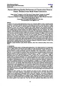
Fig. 16. Values of the total index for dumped systems.
set at the beginning of the program in a very flexible way. Remark 2. Simpler indices can be obtained discarding some of the characteristic indices and retaining those that are more important for the particular process under study. It is not necessary to use all of the characteristic indices proposed in the paper and they are given for completeness. A good control engineer having a fair knowledge of his process can do the task of selecting the proper indices very easily. Remark 3. Each characteristic index has a physical meaning, since they were selected justly from the shape of the system response, which is in turn determined by the physical nature of the system under analysis. Overshoot, undershoot, settling time, oscillations 共frequency兲, steady-state value, IAE, ISE, etc., used in the computation of the total index, are all characteristics with some physical meaning. Remark 4. The choice of the weighting factors is subjective and will depend on the particular process under investigation. But, once they are defined 共in any particular form兲 this set remains constant and will give a fair comparison of plant responses obtained from the application of different control strategies, with the objective of choosing the best control strategy for that particular set of weighting factors. Again the control engineer plays a fundamental role in the definition of the weighting factors because of the knowledge he has on the plant.
5. Simulation results and comparisons In this section the ci and I T are computed for system responses corresponding to different sec-
ond order systems and one specific pattern response shown in Table 2. All weighting factors were chosen as unity. Pattern response was obtained by applying a unit step to a second-order system with a pole at the origin and other at ⫺3, controlled by a proportional controller of gain K in the forward path. System responses were generated in the same fashion as pattern response but varying the proportional gain, as shown in Table 2. The resultant total indices are shown in Fig. 16. From Fig. 16 it is possible to see that system response 2 is the closest to the pattern response which is supported by the value of I T . In fact, the ci of r c2 are mostly greater than all the others 共closer to 1兲, or at least equal to some of those corresponding to r c1 关12兴. Although r c3 presents better indices I ts5 , I ts20 , I ts50 , I IAE , I ITAE , I ISE , I ITSE , and I an than r c2 , these cannot reverse the positive differences exhibited by r c2 in I ap , I da , I s , I spk , I sov , and I npk , mainly because r c2 does not have overshoot and r c3 has 1 关12兴. The case of oscillatory system responses with respect to the same previous pattern response ( r p1 ) was also studied. System responses were generated applying a unit step to a second-order system with a zero in ⫺4 and two poles in ⫺1 and other in ⫹5, controlled by a PID controller in the forward path with parameters K, k i , and k d . The controller transfer function is
C 共 s 兲 ⫽K⫹k i /s⫹k d s. The controller parameters are shown in Table 3 and the total indices are shown in Fig. 17. The values of the total index quantitatively indicates that system response 4 is closer to the pattern response r p1 since it has a good similarity in ci
150
Manuel A. Duarte-Mermoud, Rodrigo A. Prieto / ISA Transactions 43 (2004) 133–151
Table 3 System responses for the oscillatory cases. PID parameters
System response 4 System response 5 System response 6
Symbol
K
ki
kd
Poles
Zeros
r c4 r c5 r c6
6.0 6.5 5.5
4.0 2.5 2.0
1.0 0.0 0.0
⫺1.088⫾ j2.919; ⫺0.824 ⫺1.029⫾ j4.640; ⫺0.443 ⫺0.534⫾ j4.272; ⫺0.432
⫺4; ⫺5.236; ⫺0.764 ⫺4; ⫺0.3846 ⫺4; ⫺0.3636
I ssv , I ts20 , I ts50 , I IAE , I ITAE , I ISE , and I ITSE 关12兴 the rest being practically zero. Response 5 exhibits also values close to 1 in these same indices but the significant values are concentrated in ci I ssv , I ts50 , I IAE , I ISE , and I ITSE . Finally, response 6 does not present any ci near 1 except I ssv , due to the remarkable oscillatory transient behavior 关12兴. The previous analysis was done considering changes in the reference input 共tracking兲. If we define a pattern response of the plant under a certain type of perturbation affecting the plant 共regulation兲, the index can also be computed under the same lines as in reference changes 共tracking兲. In this case the index will deliver information about which control strategy is more insensible to that particular type of perturbation. In all the previous simulations the noiseless case was analyzed. In the case of signals corrupted by noise, the influence of the noise is taken indirectly into account since the noise will deviate the actual system response from the pattern response. These deviations caused by the noise will affect the computation of each subindex and also the total index. The noise effect will then be reflected in the total index. 6. Conclusions A method to evaluate the response behavior of dynamical systems, as compared with a pattern be-
Fig. 17. Total index for oscillatory responses.
havior, has been proposed in this paper. The system behavior is quantified by means of a performance index I T , computed from a series of characteristic indices I ci , taking into account the most important characteristics of the system response selected by the control engineer. These ci’s can be properly defined by the designer by choosing the parameters suitably. Furthermore, they can be weighted through the so-called importance factors, to emphasize some characteristics over the rest, by the judgement of the designer. The index is easy to compute and easy to interpret, which makes it useful for industrial applications to evaluate different control alternatives for a plant. The total index allows us to quantitatively decide if the behavior of certain control strategy, reflected in its system response or evolution of the controlled variable, has a good behavior compared with a desired behavior or pattern response. It also allows us to decide among different control strategies which one is the closet to the pattern response. The index calculation involves some empirical but also some analytical facts, as any good industrial measurement of the process behavior. The empirical information needed to compute the total index has to do with the particular plant under study. It is difficult to think about a universal performance index valid for any plant, unless the index is quite general and does not consider the proper characteristics, but in that case the results will be so general that no good conclusions can be drawn from the index. That is precisely the case of IAE, ITAE, ISE, and ITSE indices. Since the proposed total index consists of several characteristic indices, the benefits of this index over the classical indices are the flexibility and diversity. The flexibility is in the fact that any combination characteristic indices can be chosen with proper weighting factors. The diversity is in
Manuel A. Duarte-Mermoud, Rodrigo A. Prieto / ISA Transactions 43 (2004) 133–151
the fact that the control error is not the only information used by the index as in the classical indices. Though this index is able to satisfy some initial objectives, as to discriminate good and bad system behavior, it may not be fully ready to be used in industrial plants. More refinements and studies are needed to end up with a good industrial index. There are several other aspects that can be considered in the future to end up with a powerful tool to evaluate system behaviors. One of these aspects is to include in the analysis some frequency characteristics present in the system response either directly obtained from it or some others obtained by using some transforms 共Fourier, wavelet, etc.兲. Another subject to consider in this study is to perform a similar treatment for the control input, from time and frequency viewpoints, to include also the control effort in the final decision. Acknowledgments The research presented in this paper was funded by CONICYT-Chile, through Grant No. FONDECYT 1970351.
References 关1兴 Kuo, B., Automatic Control Systems. Prentice-Hall, Inc., Englewood Cliffs, NJ, 1995. 关2兴 Brogan, W. L., Modern Control Theory. Prentice-Hall, Inc., Englewood Cliffs, NJ, 1991. 关3兴 Ogata, K., Modern Control Engineering. PrenticeHall, Inc., Englewood Cliffs, NJ, 1993. 关4兴 Dorf, R., Modern Control Systems. Addison-Wesley Publishing Company, Inc., Reading, MA, 1989. 关5兴 Franklin, G. and Powell, D., Control of Dynamical Systems. Addison-Wesley Publishing Company, Inc., Reading, MA, 1993. 关6兴 Miller, D. E. and Davison, E. J., An adaptive controller which provides an arbitrarily good transient and steady-state response. IEEE Trans. Autom. Control AC-36, 68 – 81 共1991兲. 关7兴 Datta, A. and Ioannou, A., Performance analysis and improvement in model reference adaptive control.
关8兴 关9兴 关10兴 关11兴
关12兴
151
IEEE Trans. Autom. Control AC-39, 2370–2387 共1994兲. Ortega, R., Transient bounds of dynamic certainty equivalence adaptive controllers. Int. J. Adapt. Control Signal Process. 7, 291–295 共1993兲. Ortega, R., On Morses new adaptive controller: Parameter convergence and transient performance. IEEE Trans. Autom. Control AC-38, 1191–1202 共1993兲. Narendra, K. S. and Balakrishnan, J., Adaptive control using multiple models. IEEE Trans. Autom. Control AC-42, 171–187 共1997兲. Duarte, M. and Sepu´lveda F., Comparative cost functional for controllers 共in Spanish兲. Technical Report 96-08, Electrical Engineering Department, University of Chile, 1996. Prieto, R., Performance indices to evaluate the transient behavior of dynamical systems 共in Spanish兲. Electrical Engineer thesis, Electrical Engineering Department, University of Chile, 1998.
Manuel A. Duarte-Mermoud received the degree of Civil Electrical Engineer from the University of Chile in 1977 and the M.Sc., M.Phil., and the Ph.D. degrees, all in electrical engineering, from Yale University in 1985, 1986, and 1988, respectively. From 1977 to 1979, he worked as field engineer at Santiago Subway. In 1979 he joined the Electrical Engineering Department of University of Chile, where he is currently professor. His main research interests are in robust adaptive control 共linear and nonlinear systems兲 and system identification. Dr. Duarte is member of the IEEE and past president of ACCA, Chilean National Member Organization of IFAC.
Rodrigo A. Prieto R. received the Civil Electrical Engineering degree from the University of Chile in 1999. His research interests are in automatic control and telecommunications. He worked in automation of mining projects from 1999 to 2000 at the Contac Ingenieros Ltda. company. Currently he is working on design and operation of internet networks at the Entel S.A. company.