Performance Modeling of a Cluster of Workstations - CiteSeerX

Performance Modeling of a Cluster of Workstations Ahmed M. Mohamed, Lester Lipsky and Reda A. Ammar Dept. of Computer Science and Engineering University of Connecticut Storrs, CT 06269 Abstract Using off-the-shelf commodity workstations to build a cluster for parallel computing has become a common practice. In studying or designing a cluster of workstations one should have available a robust analytical model that includes the major parameters that determines the cluster performance. In this paper, we present such a model for evaluating a cluster’s performance. The model covers the effect of storage limitations, interconnection networks and the impact of data partitioning. The model can be used to estimate the throughput of the cluster or the expected service time of the tasks under any specific configuration. It also, can detect the bottlenecks in the system, which can lead to more effective utilization of the available resources. The model (Multi-Class Jackson Network) we use can be considered as the base line for the cluster architecture analysis because it models the system behavior without using any special task or scheduling algorithms.

Key words: Cluster Computing; Queueing Analysis; Performance Modeling; Jackson Network.

1. Introduction The development and use of cluster based computing is increasingly becoming the effective approach for solving high performance computing problems. The new trend of moving away from specialized traditional supercomputing platforms such as Cray / SGI T3E to cheap and general purpose systems consisting of loosely coupled components is expected to continue. The cluster approach gives the users flexibility in constructing, upgrading, and scaling a parallel system for a given budget, which is suitable for a large class of applications and workloads. Clearly there is a strong

need and role for the integration of performance analysis in the design of clusters and cluster based applications. However, the role of performance analysis has always lagged behind the structural and management aspects of software engineering. In the literature, there are four major approaches that can be used in performance analysis: analytical modeling, measurement, simulation and statistical prediction. Analytic models [5,14,21,23,] depend on the construction of symbolic expressions for different performance metrics. Once the expression is available, suitable mathematical functions can be applied for performing almost any kind of analysis. This approach is suitable for analyzing existing systems and future systems. The second-approach, statistical prediction [8,10], predicts execution time using past observations. Statistical methods have the advantage that they do not need any direct knowledge of the internal design of the algorithm or the machine. In direct measurement, the basic concept is to collect performance data online during the execution of the problem. An obvious disadvantage is the requirement of availability of the target computing system and fully developed and tested implementations of every potentially different design. Several worthy solutions for this approach are presented in the literature [16,22]. The relaxation of the need for the target-computing platform is perhaps the most useful characteristic of the simulation approach [1,2,7]. The simulation approach appears to be a good compromise between the accuracy of time consuming direct measurement and the mathematical approaches. However, the complexity linked to the construction of simulation models and the huge computing resources needed have often prevented the use of simulation.

In our analysis of cluster of workstations, we use the analytical modeling approach. In Section 2 we will give a brief background for some of the analytical models that have been developed for this environment. In Section 3 there will be a description of our performance model. We will present our results in Section 4.

2. Related Work The success of any performance model is dependent on how accurately the model matches the system and more importantly what insights does it provide for performance analysis. We’ll try to address some of the performance models for the clusters in this section. Petri-Nets (PN) have been heavily used for performance modeling of parallel machines as in Marsan [15], Balbo [3] and Trivedi [19,20]. Benitez [14] has used it to develop a performance model to predict the execution time of a parallel application running on a heterogeneous cluster. The model is a mix of Petri net and continuous Markov chains. Benitez used the task graph model to represent the parallel application. Given that the execution times of the tasks are exponentially distributed, then the firing rates of the transitions in the PN are exponentially distributed. This makes the reachability graph equivalent to a continuous time Markov chains (CTMC). Although the above model captures some performance parameters, it does not address the performance bottlenecks in the system like communication contention and contention due to resources sharing. Zhang, Yan and Song [23] have developed a mixed model of simulation, measurements and analytical. They used task graphs to represent the parallel application. Communication contention has been estimated by simulation. The geometric distribution is used to model the non-dedication property. The use of the deterministic distribution and the claim that it is better than the exponential distribution in modeling the service time is highly questionable. The method used to model communication contention is not accurate due to using deterministic analysis for the shared communication channel in their simulation. Modeling the non-dedication property by a geometric distribution is satisfactory but is no more

than the discrete version of the exponential distribution. Li and Antonio developed another probabilistic model in [12]. Individual task execution time distributions are assumed to be known. A probabilistic model for data transmission time is developed to model the network behavior. Three random variables are used to represent each task, start time, execution time and finish time. The analysis of this paper is general since it may be applied to any distribution. However it is hard to develop and it ignores the effect of contention. Berman in [4] introduced a model that calculates the slowdown imposed on applications in time-shared multi-user clusters. The model focuses on three kinds of slowdown: Local slowdown, Communication slowdown and Aggregate slowdown. The authors of this paper claimed that, based on their experiments, the time to execute an application in dedicated mode and the time to execute the same application under contention are directly proportional by a constant factor that they identified as the slowdown caused by contention for resources. The above model is based only on experiments so it cannot be applied in general. Also, it assumes no contention will occur in dedicated environments and ignores queueing delays. Varki [21] has developed a simple response time approximation for parallel systems with exponential service time distributions. Markov chains have been used as the analytical tool. The response time expression is derived for the system by employing alternate representations of the parallel system then equating the parameters of the alternate but equivalent representations. It is worth mentioning that the solution to this model is known analytically in order statistics. Pr (max < x) = [F(x)]n, where F(x) is probability distribution function for the tasks. In our analysis, we will focus on the architectural limitations. As we have discussed, other works that have been done in this area do not consider how these limitations can affect the performance of the system. In most of the work we have seen so far, CPU speed is the only factor that has been taken into account. We believe this is not enough. Contention in the communication links, contention in the shared disks, contention at the CPU and the way the shared data is distributed are all equally important. The model we discuss next

can model the effects of all of the above and predicts the performance of the running application.

3. The Performance Model In studying or designing a cluster of workstations one should have available a robust analytical model that includes the major parameters that determine the cluster performance. The major parameters we are modeling include communication contention, geometry configurations, time needed to access different resources and data distribution. More details can always be added to the basic model like scheduler overheads, multitasking, inhomogeneity, task dependencies…etc. Such a model is useful to get a basic understanding of how the system performs. 3.1 Application Model In this section we describe how we model the target parallel application. The parallel application (or job) can be considered to be a set of N independent, but identically distributed (iid) tasks, {t1, t2... tN}, where each task is itself made up of a sequence of requests for CPU, local data, global or remote data. The number of tasks is presumed to be much greater than the number of workstations (WS) (or PC's) that make up the cluster. We assume that each WS is made up of a CPU and a disk drive. The tasks are queued up, and the first K tasks are assigned to the cluster. When a task is finished, it is immediately replaced by another task in the queue. The set of active tasks can communicate with each other by exchanging data from each other's disks. The tasks run in parallel, but they must queue for service when they wish to access the same device. Each task consists of a finite number of instructions, either I/O instructions (need local or remote disk access) or non-I/O instructions (CPU activity). Thus the execution of the task consists of phases of computation, then I/O then computation, etc, until finished. We assume that during an I/O phase the task cannot start a new computational phase (no CPU-I/O overlap). Assume that T is the random variable that represents the running time of a task if it is alone in the system The mean execution time E(T) for task ti can be divided into three parts not including the communication cost:

E(T) = T1 + T2 + T3, Where, T1 is the expected time needed to execute non-I/O instructions locally (local CPU time). T2 is the expected time needed to execute I/O instructions locally (local Disk time). T3 is the expected time needed to execute I/O instructions (remote Disk time). We use the following parameters to represent the above components. X = T1 + T2. C is the fraction of local time that the task spends at the local CPU. T1 = C * X . T2 = (1 – C ) * X. T3 = Y. So we can write T as: E(T) = C * X + ( 1 – C ) * X + Y. All of the above parameters assume no contention. The performance model uses these parameters to calculate the effect of contention when more than one task is running in the cluster. For simplicity we will normalize the task expected execution time. Therefore, E(T) = 1 and hence, Y = 1 - X. 3.2 System Model In general a cluster can be considered as (either homogeneous or heterogeneous) a distributed computing platform. It can be dedicated, where the parallel program has full control over the whole cluster, or undedicated where the parallel program uses the full computational power of the nodes only when they are not used by a local owner. When a node is busy, there should be an agreement between the owner of the node and the cluster about the percentage of computational power that the node will provide to the cluster. The network model assumes the transmission time is modeled according to a probabilistic distribution (Exponential). Two different architectures are considered: 1. Centralized Storage. In this model there is a central storage node and all nodes contact this central node when they request global data. 2. Distributed Storage. Here, the required global data is distributed among all of the nodes.

3.3 Modeling The Cluster We believe that a system with such a configuration should always be analyzed first by a Network queueing model (Jackson network model). This is a very good way of identifying and organizing parameters and locating bottlenecks, even if the exponential assumptions and independence of tasks are not satisfied. If applied correctly, Jackson network models are known to be very reliable under very light load or very heavy load. General exponential queueing network models were first solved by Jackson[11] and by Gordon and Newell[9]. Buzen[5,6] developed the idea of using the G function as an efficient tool for analyzing the performance. Muntz, Chandy and Basket [18] developed many of the basic notions concerning several job streams, as well as some notions concerning non-exponential holding times. Moore [17] introduced the use of generating functions for the treatment of network queueing models. Our analysis for the performance of the computing cluster will use the generating functions for multiple classes queueing networks. Each of the k active tasks resides in its own CPU. Thus we put each task in its own class. (e.g., task 1 does not use CPU 2, 3 or 4. but uses the other disks as remote) 3.3.1 Example for a Central Cluster. In this model, all of the tasks go to central server asking for data, each task takes Y units of time to get its data if there is no contention. Each task will spend C*X units of time in average at its local CPU and (1 – C)*X units of time an average at its local disk. Each node will be charged B*Y units of time to use the shared communication link. The task resides in the central server does not go to the shared communication link when it needs to access its disk. E=

0 0 0 0 0 C*X Y+(1- C)*X 0  Y C*X (1- C)*X 0 0 0 0 0 0 Y 0 0 C*X (1- C)*X 0 0  Y 0 0 0 0 C*X (1- C)*X  0

0   B*Y B*Y  B*Y

The above matrix represents a four-node and four classes central cluster, Eij is the mean time task i needs on server j in case of no contention(if the task is alone in the cluster). Each row represents a task or a class. The columns represents the nodes, the first column is the CPU of the central server and

the second column is its disk, then each two columns represent a node the first for the CPU and the second for the disk. The last column is the communication cost for each task. To model the cost of the scheduler overhead, we would use another parameter and charge that to the one or more CPU’s. 3.4 Basic Assumptions 1. Exponential Distribution: We assume that the service time of each server (CPU or Disk) and the rate of requesting data (I/O) are exponentially distributed. The assumption of exponential service time is a venerable assumption in all branches of queueing theory. Since the queue length in any node does not become large, the exponential distribution will give a very good approximation even if the actual distribution is not exponential. 2. Time Sharing: We assume that the processor sharing property is applied in each server. Since we assume exponential service time, we can say our analysis is also valid if the queue discipline is FIFO. 3. Memory Limitation: We assume that each node has enough amount of memory to for its own local work. If the node does not have enough memory, an overhead for context switching would be added. This can be modeled too by introducing another parameter to be charged to the CPU. 4. Communication: We assume non-blocking send and blocking receive (you have to wait for the requested data before you can resume work). 3.5 The Algorithm Assume we have M nodes and K classes then, the generating function G for this model can be calculated from the following formula[6] (see e.g., [13] for algorithmic details): GM(N1, N2, ……..,NK) = GM-1(N1, N2, ……..,NK) + X1M GM(N1 – 1, N2, …….., NK) + X2M GM (N1, N2 – 1, …….., NK) + …… + XKM GM (N1, N2,N3, ……..,NK – 1) The performance metric used here is the throughput, which can be calculated as following: Qi=GM(N1, N2,,……..,NK)/GM (N1, N2, …..,NK)

Where, Qi is the throughout of class i. Ni is the number of customers in class i. In our case it is equal one (one task per node). Xij is the time spent by class i in server j. In our analysis we assumed that the tasks are queued up, and the first K tasks are assigned to the cluster (Ni = 1). When a task is finished, it is immediately replaced by another task in the queue. If one desires to have more than one task to share node i, then change the value of Ni from 1 to the number of tasks that share node i.

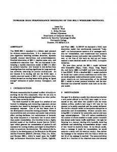
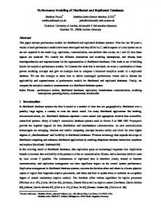
4. Analysis and Results In the following section we will study the performance behavior of both the distributed and central cluster under different configurations. We modeled both the central and the distributed clusters for three different sizes (5, 8 and 10) WS’s. In figures 1.a and 1.b we ignored the communication cost (B = 0) to check how the contention at the shared disks may affect the performance of the cluster. In all figures we present, we use the average throughput of the cluster. The average throughput is the sum of the throughput of all nodes divided by the number of nodes in the cluster. It is clear from figure 1.a how the contention at the central disk affects the average throughput of the central cluster (it would equal one if no contention occurred). For example if we have an 8 node central cluster and we spend 25 % of the task time at the central disk, the average throughput of the cluster will be decreased by 50%. Meanwhile, the distributed cluster scales very well if we can ignore the communication cost. In other words the cluster size has small effect on the contention of the shared disks of the distributed cluster if we ignore the communication cost. We can use these graphs to estimate the throughput of the cluster or the expected service time of the tasks under any specific configuration. In figures 2.a and 2.b we added the communication cost and we assume that B = 1. We see in fig. 2.a how the contention at the communication channel can hurt the distributed cluster, now it is no better than the central cluster. There is a serious degradation in the average throughput of the cluster. In figure 2.c we see the

probability of the communication channel to be busy vs. the amount of local work. As we increase the remote load(decrease the local work) the probability for the channel to be busy increases. For M = 10 and M = 8, the channel saturates when the task spends 25% of its time remotely. In figure 2.d, for the central cluster, the probability for the central disk to be busy is always greater than the channel. So, the contention at the central disk is the bottleneck for the central cluster not the communication network. In figures 3.a and 3.b we increased the local disk load, while decrease the CPU load, but both systems have almost the same behavior. The reason is the bottleneck in each is still the same (communication for distributed cluster and central disk for central cluster) without any modification, so increasing the local disk load did not change the average throughput in both systems. Obviously these calculation are highly dependent upon the values of C, X and B. In designing a real cluster these parameters must be estimated with some accuracy for the calculation to be applicable.

5. Conclusion The development and use of cluster based computing is increasingly becoming an effective approach for solving high performance computing problems. We believe that understanding the performance limitations of such environment will help in using it efficiently. In this paper, we introduced an analytical performance model that can predict the behavior of the cluster under different circumstances. The model is flexible and can be adapted to many platforms. We modeled the degradation in the performance that occur due to the contention in the communication channel and shared disks. We showed how these contentions can affect the performance of the cluster. The model can also predict the contention at the CPU or the local memory if needed with minor modifications.

6. REFERENCES [1] D. Abramson, J. Giddy, “ Nimrod: Tool for Performing Simulation using Distributed Workstations,” The 4th HPDC, Aug. 1995. [2] K. Aida, U. Nagashima, “Overview of a Performance Evaluation System for Global Scheduling Algorithms,”

Proc. of the 8th IEEE Inter. Symposium on High Performance Distributed Computing, pp. 97-104, 1999. [3] G. Balbo, G. Serazzi, “Asymptotic Analysis of Multiclass Closed Queueing Networks: Multiple Bottlenecks”, Performance Evaluation, Vol. 30, pp. 115152, 1997. [4] F. Berman, S. M. Figueira, “A Slowdown Model for Applications on Time-shared Clusters of Workstations,” IEEE Transaction on Parallel and Distributed Systems, vol.12, pp. 653-670, Jun 2001. [5] J. P. Buzen, “Queueing Network Models of Multiprogramming”, Ph.D. Thesis, Div. Of Engr. and Physics, Harvard University, 1971. [6] J. Buzen, “Computational Algorithms for Closed Queueing”, Comm. ACM, Vol 16, No. 9, Sep 1973. [7] P. Dinda, “Online Prediction of the Running Time of Tasks,” 10th IEEE International Symposium on High Performance Distributed Computing, pp. 383-394, 2001 [8] I. Foster, W. Smith, V. Taylor, “Predicting Application Run Times Using Historical Information,” Proc. of IPPS/SPDP'98 Workshop, pp. 122-142, 1998. [9] W. J. Gordon, G. Newell,”Closed Queueing Systems with Exponential Servers”, JORSA, Vol. 15, pp. 254-265, !967. [10] M. A. Iverson, F. Ozguner, L. C. Potter, “Statistical Prediction of Task Execution Times Through Analytic Benchmarking for Scheduling in a Heterogeneous Environment,” IEEE Transactions on Computers, vol. 48, no. 12, pp. 1374-1379. Dec. 1999. [11] J. Jackson, ”Jopshop-Like Queueing Systems”, J. TIMS, Vol. 10, pp. 131-142, 1963. [12] Y. Li, J. Antonio, ”Estimating the Execution Time Distribution for a Task Graph in a Heterogeneous Computing System,” Proc. of the 6th HCW 1997, pp. 172-184, 1997. [13] Lester Lipsky, J. D. Church,” Applications of a Queueing Network Model for a Computer System”, ACM Computing Surveys (CSUR), Vol. 9, Issue 3, Sep. 1977. [14] N. Benitez, A. McSpadden, “Stochastic Petri Nets Applied to the Performance Evaluation of Static Task allocations in Heterogeneous Computing Environments,” Proceedings of the 6th Heterogeneous Computing Workshop, pp. 185-194, 1997. [15] M. Marsan, G.Balbo, G.Conte, “A Class of Generalized Stochastic Petri Nets for the Performance Evaluation of Multiprocessor Systems'', ACM Transactions on Computer Systems, Vol.2, n.2, , pp.93122 , May 1984 [16] B. Mohr, A. Malony, “Speedy: An Integrated Performance Extrapolation Tool For pC++ Programs,” Proc. of Joint Conference Performance Tools, pp. 254268, 1995.

[17] F. Moore, “Computational Model of a Closed Queueing Network with Exponential Servers”, IBM J. of Res. And Develop., pp. 567-572, Nov. 1962. [18] R. Muntz, F. Baskett, K. Chandy,” Open, closed and Mixed Networks of Queues with Different Classes of Customers”, JACM, Vol. 22, pp. 248-260, Apr 1975. [19] K. Trivedi, Oliver C. Ibe, Choi, “ Performance Evaluation of Client-Server Systems,” IEEE Transaction on Parallel and Distributed Systems, Vol. 4, pp. 12171229, Nov. 1993. [20] K. S. Trivedi, A. Puliafito, M. Scarpa, “Petri Nets with k-Simultaneously Enabled Generally Distributed Timed Transitions,” Performance Evaluation, Vol. 32, No.1, pp. 1-34, Feb. 1998 [21] E. Varki, “Response Time Analysis of Parallel Computer and Storage Systems,” IEEE Transaction on Parallel and Distributed Systems, vol. 12, no. 11, pp. 1146-1161, Nov. 2001. [22] R. Wolski, N. T. Spring, J. Hayes, “The Network Weather Service: A Distributed Resource Performance Forecasting Service for Metacomputing,” J. Future Generation Computer Systems, vol.15, no.5-6, pp. 757-768, 1999. [23] Y. Yan, X. Zhang, Y. Song, “An Effective Performance Prediction Model for Parallel Computing on Non-dedicated Heterogeneous Networks of Workstations,” J. of Parallel and Distributed Computing, vol.38, no.1, pp. 63-80, 1996.

M5 M8

Distributed Cluster Fig 1.a

0. 1

M =8

X

0. 1

0. 25

0. 4

0. 7

0. 55

M =5

Distributed Cluster Fig 2.a

Central Cluster Fig. 2.b C = 0.9, B = 1

C = 0.9, B = 1

1.2 M = 10 D

1

M = 10 Ch

M = 10

0.8

M=8

0.6

M = 8 Ch

0.4

M=5D

P

P

0. 25

M =10

1

0. 1

0. 25

0. 4

0. 55

0. 7

M =5

C = 0.9, B = 1

1.2 1 0.8 0.6 0.4 0.2 0 0. 85

M =8

Q

M =10

0. 85

1

Q

C = 0.9, B = 1

1.2 1 0.8 0.6 0.4 0.2 0

X

Central Cluster Fig. 1.b

1.2 1 0.8 0.6 0.4 0.2 0 X

0. 4

0. 7

1

0. 55

M 10

0. 1

X

0. 25

0. 4

0. 55

0. 7

0. 85

M = 10

C = 0.9

1.2 1 0.8 0.6 0.4 0.2 0

0. 85

M =8

1

Q

M =5

0.6 0.4 0.2 0

Q

C = 0.9

1.2 1 0.8

M=5

M=8D

M = 5 Ch

0.2

Fig 2.c C = 0.5, B = 1

Distributed Cluster Fig 3.a

0.1

0.2

0.3

0.4

M =8

Central Cluster Fig. 3.b

0. 1

X

0. 25

0. 4

0. 55

M =5

0. 7

X

M = 10

0. 85

M=5

1

M=8

1.2 1 0.8 0.6 0.4 0.2 0

Q

M =10

0.6

1 0. 9 0. 8 0. 7 0. 6 0. 5 0. 4 0. 3 0. 2 0. 1

Q

1

0

0.5

C = 0.5, B = 1

0.8

0.2

X

Fig. 2.d

1.2

0.4

0.6

0.7

0.8

X

0.9

1

0. 9 0. 8 0. 7 0. 6 0. 5 0. 4 0. 3 0. 2 0. 1

1

0