Switch. Master Subnet Manager. Router. Figure 1. Physical Model of Subnet Management. The SMP header defines the operation to be performed by the SM.
Performance Modeling of Subnet Management on Fat Tree InfiniBand Networks using OpenSM Abhinav Vishnu
�
Amith R Mamidala Hyun-Wook Jin Dhabaleswar K. Panda Department of Computer Science and Engineering The Ohio State University Columbus, OH 43210 vishnu, mamidala, jinhy, panda @cse.ohio-state.edu �
Abstract
performance computing environments by using Clusters. It combines the computational power of commodity PCs and the communication performance of high speed network interconnects. Fat Trees [6] are being used as a primary interconnection topology for building large scale clusters. Recently, InfiniBand Architecture [5] has been proposed as the next generation interconnect for I/O and inter-process communication. Due to its open standard and high performance, InfiniBand is becoming increasingly popular for cluster computing. InfiniBand defines a technology for interconnecting the I/O nodes with the processing nodes, which forms a System Area Network (SAN). The end nodes are connected to each other in a switched point-to-point fashion. The end nodes can have one or more Channel Adapters to connect to the network. InfiniBand specifies a small number of management classes. It specifies a Subnet Management mechanism which monitors the state of the subnet and takes appropriate steps to assimilate topology changes in a smooth fashion. It specifies an entity called Subnet Manager (SM) which is in charge of discovery, configuration and maintainence of the subnet. A lot of simulation based studies have been presented in the recent past to evaluate the subnet management mechanism [3] [4]. However, these studies are based on irregular topology networks and lack the management model on regular topologies using actual implementations. In this paper, we take up the challenge of modeling subnet management mechanism for Fat Tree InfiniBand networks using OpenSM [1]. We present the timings for various subnet management phases in InfiniBand [3] such as topology discovery, path computation and path distribution for large scale fat tree InfiniBand networks. We also present the timings on a small scale InfiniBand cluster with different configurations to understand the behaviour of subnet manager. We verify our model with the basic set of results ob-
InfiniBand is becoming increasingly popular in the area of cluster computing due to its open standard and high performance. Fat Tree is a primary interconnection topology for building large scale InfiniBand clusters. Instead of using a shared bus approach, InfiniBand employs an arbitrary switched point-to-point topology. In order to manage the subnet, InfiniBand specifies a basic management infrastructure responsible for discovery, configuration and maintaining the active state of the network. In the literature, simulation studies have been done on irregular topologies to characterize the subnet management mechanism. However, there is no study to model subnet management mechanism on regular topologies using actual implementations. In this paper, we take up the challenge of modeling subnet management mechanism for Fat Tree InfiniBand networks using a popular subnet manager OpenSM. We present the timings for various subnet management phases namely topology discovery, path computation and path distribution for large scale fat tree InfiniBand subnets and present basic performance evaluation on small scale InfiniBand cluster. We verify our model with the basic set of results obtained, and present the results for the model by varying different parameters on Fat Trees.
1 Introduction In the past couple of years, the computational power of commodity PCs has been doubling about every eighteen months. At the same time, commodity network interconnects that provide low latency and high bandwidth are also emerging. This trend makes it very promising to build high �
This research is supported in part by Department of Energy’s Grant #DE-FC02-01ER25506, National Science Foundation’s grants #CCR0204429 and #CCR-0311542, and grants from Intel and Mellanox, Inc.
1
tained, and present the results for the model by varying different parameters on Fat Trees. The rest of the paper is organized as follows: In Section 2, we provide background information for InfiniBand, Subnet Management and Fat Trees. In Section 3, we discuss various phases in subnet management. In Section 4, we present the timings for various management phases using OpenSM for small scale InfiniBand network configurations. In Section 5, we present the subnet management model on Fat Tree Networks. In Section 6, we show the performance results using our management model and validate it by using the timings from section 4. In section 7, we present the related work of this paper. In section 8, we conclude and discuss the future directions.
Direct routed SMPs contain the information of the output port to which they need to be fowarded to at each intermediate hop. Direct routed SMPs are used during the subnet discovery before the subnet initialization. LID routed SMPs have lesser overhead than direct routed SMPs, because the direct routed SMPs have to be processed at each intermediate SMI. Master Subnet Manager
SMA Switch
2 Background In this section, we provide background information for our work. We first provide a brief introduction of InfiniBand Subnet Management machanism and then discuss about fat tree topologies used in building large scale clusters.
2.1 InfiniBand Subnet Management The InfiniBand Architecture (IBA) [5] defines a switched network fabric for interconnecting processing nodes and I/O nodes. It provides a communication and management infrastructure for inter-processor communication and I/O. In an InfiniBand network, processing nodes and I/O nodes are connected to the fabric by Channel Adapters (CA). Host Channel Adapter (HCA) sit on processing nodes. InfiniBand defines a small number of management classes. The Subnet Management class defines an entity called Subnet Manager (SM), which is in charge of discovering, configuring, activating and managing the subnet. The subnet manager can reside in any subnet device (Switch, Router or Channel Adapter (CA)). By using the subnet management interface (SMI), SM can exchange control packets with the subnet management agents (SMA) present in every subnet device. The SMI is associated to an internal management port in switches, or to a physical port in the rest of the devices. Figure 1 shows the physical model of the subnet management. The control packets used by subnet management are called subnet management packets (SMPs). Each SMP consists of 256 bytes of data. SMPs use the Unreliable Datagram service, which contain a key to authenticate the sender and use the management virtual lane (VL15). The SMPs can be classified into LID routed and Direct routed SMPs. LID routed SMPs are routed by switches by a table lookup of the forwarding table. They are mostly used to check the status of active ports in the subnet. The data packets are routed in the same way as LID routed SMPs.
SMA
SMA
SMA
Router
Switch
Switch
SMA
SMA
SMA
SMA
Channel Adapter
Channel Adapter
Channel Adapter
Channel Adapter
Figure 1. Physical Model of Subnet Management
The SMP header defines the operation to be performed by the SM. These subnet management operations are : Get, Set, GetResp, Trap and TrapRepress. The Get operation is used to get the information about the CA, Switch or a Router port. The Set operation is used by the subnet manager to set the attributes of a port at the end of the subnet discovery. The GetResp operation is the response to the Get SMP of a subnet manager. The subnet manager performs a sweep to discover the subnet. In addition to sweeping, a switch may optionally inform the SM about the change of the state of a local node by sending a Trap notice SMP. In addition, the SMA may periodically repeat the Trap message until it receives a notification from the SM to stop the trap by sending a TrapRepress message. The SMI injects SMPs generated by the SM and SMAs into the network. In addition, it validates and delivers incoming SMPs. SMAs are passive management entities. SMAs process received SMPs, respond to the SM, and configure local components according to the management information received. The received SMPs can contain information about LID assignment of physical ports, the state of the ports, and the number of data operational VLs. Other SMPs are used to update the local forwarding table, the SL to VL mapping table, and the VL arbitration tables. In switches, the SMA 2
3.1 Subnet Discovery
can send traps to the SM to notify the change in state of a local port. SM is a management entity which manages the subnet. With the help of SMPs the SM is able to discover the subnet topology, configure subnet ports and switches, and receive traps from SMAs. In addition to the Master SM, multiple Subnet Managers may be present in the subnet. However, only one of them can be the master SM. The rest of the Subnet Managers are Standby SMs. The standby SMs periodically poll on the master SM and wait for a successful response. In case of failure of the Master SM, one of the Standy SMs becomes the master SM.
In order to start the discovery process, the SM sends a Get SMP message to its local node using an empty directed path, and waits for the response. Upon receipt of the response, it sends direct routed SMPs with additive depth to facilitate the discovery of other nodes in the subnet and so on. During the discovery process, the SM configures the port attributes, sending Set SMPs to the CA and switch ports. A subnet manager may decide to send multiple exploration SMPs to discover the subnet at any point in time [3]. However, OpenSM [1] uses one outstanding SMP for exploration, in order to perform controlled breadth first search. The subnet discovery phase can be characterized into multiple phases:
2.2 Fat Tree Topology
Setup time for switch ports Setup time for CA ports OpenSM sends a Get SMP with NodeInfo attribute to get the kind of end node (Switch, CA or Router) and a Get SMP with PortInfo to get the port attributes. It sends a Set SMP to set the LIDs and other port attributes. OpenSM provides an option of Trap based subnet discovery. In order to allow a switch to notify the subnet manager about topology change, SM initializes every port on the switch, even though it may not have any active connection with a CA.
Figure 2. (a)Traditional Binary Tree (b)Binary Fat Tree
Fat tree is a general purpose interconnection topology, which is used for effective utilization of hardware resource devoted to communication. Fat trees differ from the traditional trees in the amount of resource bandwidth available at different levels of the tree. In traditional trees, the link bandwidth is fixed at all levels of the tree. Due to this configuration, there is congestion near the root of the tree. In a Fat tree, the link bandwidth is higher near the root in comparison to the leaves. For a complete Fat tree, the link bandwidth doubles at every level, starting from the leaves. Figure 2 shows the difference between a traditional fat tree and a binary fat tree. In a Fat tree based interconnection network, leaf nodes represent processors, internal nodes represent switches, and edges correspond to bidirectional links between parents and children.
3.2 Path Computation Once the topological information of the subnet is received, the subnet manager needs to compute the paths for data packets to follow in order to reach the destinations. This would constitute the computation of forwarding tables. The InfiniBand specification does not impose any specific routing algorithm for the path computation. When multiple paths are available between the end nodes, OpenSM selects the one with the least number of hops. In case of a tie, one of the available paths is chosen randomly. We characterize the path computation time as a function of the number of end nodes in section 5.
3.3 Path Distribution
3 Subnet Management Mechanism
Once the paths to every device in the subnet have been computed, the forwarding tables at each switch need to be configured for routing of data packets. InfiniBand specification clearly defines the SMPs for updation of switch forwarding tables. However, the update order is not specified. OpenSM [1] performs the forwarding table configuration phase once the path computation phase is complete. This policy is optimal, because during the complete subnet discovery, nodes are not ready for communication, unless the whole subnet is in ACTIVE state.
In this section, we present various phases of subnet management in InfiniBand. A more detailed description is present in [3]. The topology discovery phase consists of sending direct routed SMPs to every port in the subnet and processing the responses. The path computation phase comprises of computing valid paths between each pair of end nodes. The path distribution phase consists of configuring forwarding table on switches. 3
4 OpenSM Basic Performance
are connected to end nodes, OpenSM needs to setup all the switch ports to facilitate trap based discovery. Hence, as shown in Figure 7, the switch setup time remains constant with increasing the number of end nodes.
In this section, we present the performance of OpenSM on a small scale InfiniBand cluster. We consider a set of configurations: A 1-switch configuration, which consists of an 8-port crossbar switch and 6-switch configuration which consists of six 8-port crossbar switch blocks connected in a fashion as shown in the Figure 3.
4.1.1 Subnet Discovery
90 16−Port Switch
1-switch 6-switch
80
Switch Block
Switch Block
Switch Block
70
Switch Block
Time (ms)
Switch Block
Switch Block
60 50 40 30
8
7
6
5
4
3
2
20
1
10 1
Figure 3. The 6-switch Configuration
2 4 Number of Nodes
For the 6-switch configuration, in order to take the results for k nodes, the nodes numbered from 1 to k were used. An x represents an unused port in the switch.
Figure 5. Path Computation Time
The channel adapter setup time remains almost the same for both 1-switch and 6-switch configurations. There is a slight difference for 8 nodes on 1-switch in comparison with the 6-switch configuration as shown in Figure 6. This is due to the difference in number of hops and hence increased SMI processing for the 6-switch configuration. However, SMI processing time is much smaller in comparison to the total setup time and hence we ignore its effect to simplify the performance modeling in section 5. Once the topology discovery is complete, OpenSM needs to configure valid routes between end nodes.
4.1 Total Discovery time Figure 4 shows the total discovery time for multiple switch configurations. The total discovery time increases with the increasing number of nodes. We divide this time in multiple management phases and show the results in the following sections. 140
1-switch 6-switch
120
80 60
Time (ms)
Time (ms)
100
40 20 0 1
2 4 Number of Nodes
8
8
6 5.5 5 4.5 4 3.5 3 2.5 2 1.5 1 0.5
1-switch 6-switch
1
Figure 4. Total Discovery time
We notice that the total discovery time for any of the configurations above does not increase exactly in a linear fashion. This is because, even if a subset of switch ports
2 4 Number of Nodes
Figure 6. Channel Adapter Setup time
4
8
40
4
1-switch 6-switch
35
3 Time (ms)
30 Time (ms)
1-switch 6-switch
3.5
25 20 15
2.5 2 1.5
10
1
5
0.5 0 1
2 4 Number of Nodes
8
1
Figure 7. Switch Setup Time
because, the per table entry overhead is very small. Each table entry occupies 16-bit for LID and 8-bit for the forwarding port. Hence only one Set SMP with LinearForward�������� � ingTable attribute is required for every nodes per switch. In our experimentation platform, the MTU is 2048 bytes and thus only one Set SMP is required for 8 nodes.
We calculate the overhead of path computation in terms of the number of end nodes in the subnet. From Figure 8 we can clearly see, that the path computation overhead increases almost linearly with the number of end nodes. The path distribution phase consists of distributing the forwarding tables to the switches in the subnet. Clearly, it is dependent on the number of switches and number of entries which need to be configured per switch. As shown in Figure 9, for a 6-switch configuration, for the same number of nodes, the path distribution time is higher, because the SM needs to configure the forwarding table on 6 switches instead of 1-switch.
5 Subnet Management Model on Fat Tree Networks Routing in a complete Fat tree is simple as there exists a unique shortest path between every pair of processing nodes [7]. However, the requirement of increasing arity of switches makes the physical implementation of switchbased Fat tree infeasible. To solve this problem, some alternatives have been proposed to construct fat trees using constant size elements or use fixed arity switches. Based on the fixed arity of the communication switches to construct a fat tree network, we use an m-port n-tree configuration of a fat tree in our analysis and evaluation. Given an m-port n-tree, it has the following characteristics.
1-switch 6-switch
80 70 Time (ms)
8
Figure 9. Path Distribution time
4.1.2 Path Computation
90
2 4 Number of Nodes
60 50 40
�
The tree consists of ������ ���� processing nodes and � �� ������ ��� ���
!� �#"%$ communication switches
30 20 10 1
2 4 Number of Nodes
Each communication switch has m communication ports
8
Before the end nodes can communicate with each other, the SM needs to configure the routes for the intermediate switches and end nodes after the subnet discovery. As mentioned before, to start the discovery process, the SM first sends a Get(NodeInfo) to its local node (using an empty directed path) and waits for a response. Each time the SM receives a response GetResp SMP, it sends another SMP by increasing the length of the direct route. The SM sends one
Figure 8. Path Computation Time
4.1.3 Path Distribution It is interesting to see that the path distribution time remains almost constant with increasing number of nodes. This is 5
SMP per port with AttributeID as NodeInfo to determine the nature of the port and with AttributeID as PortInfo to get information about the port. Then it sends Set SMPs to configure the port attributes of discovered devices. Thus the total number of Get SMPs is the sum of SMPs with NodeInfo and PortInfo AttributeID. Let GetS(m,n) denote the number of Get SMPs generated during topology discovery, let �������� �� �� ������� � , ��� ��������� ������ ��� ����� � � be the Get SMPs with NodeInfo and PortInfo attributes respectively. Thus the number of SMPs generated during the discovery algorithm can be calculated as a function of m and n:
We now present the timings for various phases in the subnet management. We define � CIH , �J��5 and �J� H as the time taken for topology discovery, path computation and path distribution phases, respectively. The topology discovery time can be calculated in terms of the processing time for Get and Set SMPs. From the results of section 4, we can conclude that the processing time for both type of SMPs is nearly same. In addition, each of these SMPs needs to be processed at each intermediate SMI. However, intermediate SMI processing time is much smaller than the end SMI processing time, hence we ignore the intermediate SMI processing time to simplify the model. Hence the topology discovery time can be summarized as:
������ ����� � �� �������� � �� �! ��� ����� � � "#������ �� ������ ��� ������� � (1)
�JCIH �������