Efficient Network Topology Measurement Based on Ingress to Subnet Reachability Ibrahim Ethem Coskun
Muhammed Abdullah Canbaz
Mehmet Hadi Gunes
University of Nevada, Reno
[email protected]
University of Nevada, Reno
[email protected]
University of Nevada, Reno
[email protected]
Abstract—Internet topology measurement studies rely on a few vantage points to trace towards a large number of destinations. Such traces contain significant overlaps, which increase the measurement traffic and duration. As there is considerable redundancy in the generated measurement probes, researchers have been exploring probe reduction approaches with minimal loss of the topological information. To decrease the probing overhead, in this paper, we propose InSub probing technique which relies on ingress points of the Autonomous System (AS) towards the target subnetworks. To identify ingress points for each subnetwork of the target AS, we first probe the subnet prefixes announced via BGP. After identifying the ingress points of subnetworks, the subsequent probing is conducted based on the vantage point reachability of the ingresses. As shown in an experimental study with 10 ASes, InSub approach considerably reduces the probing overhead while minimizing the loss of topological information.
I. I NTRODUCTION Internet consists of tens of thousands of distinct ASes interconnected with each other. As each AS has it’s own network deployment practices and routing policies, the characteristics of the overall network is an open question that researchers have been tackling with [1]. Network measurement helps us better understand the characteristics of the Internet and improve Internet topology and services along with management of large scale ISPs [2]. Internet topology measurement involves active measurements where probe packets are used to collect information about network devices. In general, a large number of traces are used to collect path information about paths from vantage points to a given set of destinations. It is important to have a good vantage point distribution over the Internet to obtain a non-biased sample topology [3]. One of the challenges faced when mapping a network is the significantly redundant trace traffic [4]. Minimizing the redundant probing is also important in terms of the time it takes to complete a measurement campaign as well as the time for processing the collected data. High volumes of probing traffic towards a destination AS might trigger firewalls and be blocked by the destination AS [5]. Thereby, minimizing redundant probes is important not only in the sense of efficiency but also to abstain from involuntary disruption of the measured networks. In this paper, we present an AS topology measurement approach, named InSub, that focuses on identifying the ingress points of the announced subnet prefixes of the AS with respect to available vantage points. In the InSub approach, we first
identify the ingress points of the destination AS for each subnet prefix announced via BGP from all vantage points. Then, we probe known subnet IP addresses through each ingress by selecting a subset of the vantage points. The proposed InSub approach considerably diminishes the redundant probing as the vantage points that probe a subnet prefix through the same ingress are eliminated. In our evaluations, we observe that InSub approach reduces the number of probes in the destination AS by more than half, similar to the commonly utilized tree based approach [4]. In the rest of the paper, we first present related work in Section II. We present the InSub probe reduction approach that utilizes ingress to subnet prefix reachability of ASes in Section III. We then present experimental results in Section IV and conclude with Section V. II. R ELATED W ORK In this section, we provide a brief overview of current approaches to network probe overhead reduction. Rocketfuel was one of the earlier systems implementing a probe reduction approach, named directed probing [6]. Directed probing is based on recognizing transit traceroutes that pass through a network by identifying the entry and exit points of the traces based on BGP announcements collected from the RouteViews [7]. As Rocketfuel tries to minimize redundant crossing of an AS based on the BGP information, it misses the actual link level connectivity and hence potential topological views. Scriptroute handles inter-monitor redundancy by reverse path tree approach, which considers the tree built around a destination node when probed from multiple vantage points [8]. When a trace towards a destination is completed by one of the vantage points, the information about the visited IPs in the trace is embedded in the measurement script of other vantage points. If the script recognizes that it has reached part of an already traversed path, then it stops. However, this system does not deal with intra-monitor redundancy. Doubletree approach observes the tree-like structure of Internet routes around vantage points and destinations and deals with both intra- and inter- monitor redundancies [4]. Doubletree first decides a tuning parameter to estimate mid point for a path. Then, a vantage point probes both forwards toward the destination and backwards toward the vantage point starting from the mid point. Each vantage point adds the
traversed paths to a local and a global stop sets. However, as the vantage points need to share information about the visited paths, this approach involves control traffic between the vantage points which adds to the communication overhead and adds delay to the measurement campaign. Ingress point spreading approach integrates Subnet Centric Probing, Interface Set Cover, and Vantage Point Spreading [9]. Subnet Centric Probing utilizes subnetting of IPs and expands the Doubletree by eliminating the mid point parameter. By using notional prefix ingresses and hop number of the first router interface that followed by an IP within the target prefix, IPS computes a per-destination rank ordered list of vantage points. After selection of the vantage points, IPS probes the destination IPs by spreading the targets among the vantage points. Similar to Doubletree, however, the approach involves coordination traffic among vantage points. Cheleby deals with intra- and inter- monitor redundancies by collecting partial traces from the ingress points of destination ASes and tracing each destination from each of the geographically clustered vantage points [1]. The approach reduces redundant probes without coordination traffic between vantage points. The proposed InSub approach, extends the ingress point spreading approach so that it does not involve coordination traffic among vantage points similar to the Cheleby system. III. I N S UB : I NGRESS TO S UBNET R EACHABILITY BASED P ROBE R EDUCTION In this section, we present Insub probe reduction approach which is based on the detection of ingress points of subnet prefixes with respect to the vantage points. InSub probe reduction approach focuses on two essential information. First, it discovers the ingress points of subnet prefixes announced by the destination AS. Second, it efficiently distributes the probing of subnet IPs to the vantage points based on the identified ingress points of the subnetworks. A. Ingress Point Identification (IPI) We first identify ingress points of subnet prefixes from each vantage point. To this end, we gather BGP announcements (e.g., from RIPE-NCC [10]) and filter the data by removing the overlapping smaller sized subnet prefixes (i.e., with larger CIDR). If there are multiple overlapping prefixes announced by an AS, we only use the larger subnet announcement to identify the ingresses. When tracing toward a destination AS, probes to the preceding ASes are typically redundant as they overlap in their path to reach the destination AS. Hence, in order to address intramonitor redundancy, we minimize probes to routers outside the destination AS similar to the Cheleby approach that sets the initial TTL of traceroute based on the previous traces toward the AS [1]. Starting path traces from a certain hop distance from vantage points tries to direct probes towards network regions that would be within the destination AS. For each vantage point, we initialize the first hop of the path trace towards a target IP starting from T T Lmin , which is typically 1 but can be set to a higher value to bypass internal
routers. We then set the initial TTL value of the rest of the path traces towards the other IPs of the subnet prefix based on the hop distance Hi of the ingress point that the first trace revealed. If any of the subsequent traces to the AS have an ingress hop distance Hi greater than the previously set TTL, then we do not change the initial TTL value. However, if any of the ingress hop distance Hi of subsequent traces to the AS is smaller than the previously set TTL value, then we probe backwards until a new ingress point is identified, and update the initial TTL value of subsequent traces to Hi . For example, assume we have a network as shown in Figure 1. We send the first trace to Target IP1, and identify the ingress point at the 5th hop from the vantage point VP. We send the second trace to IP2 with the initial TTL value of 5 (i.e., Hi = 5). The second trace starts from router ’A’ while the ingress point for IP2 is at the 7th hop. In this case, TTL value is kept at 5. When we start the third trace from the 5th hop at route B, we cannot observe the ingress point. Hence, we probe backwards toward the VP until the ingress point is observed at hop distance 3. Hence, we update the initial TTL value for the rest of the traces to 3 (i.e., Hi = 3). Finally, the fourth trace to IP4 starts from 3rd hop at router ’C’. In order to determine the ingress point of a subnet prefix from a vantage point, we probe the first and the last IPs in each announced subnet prefix of destination AS. We then compare the identified ingress points of the first and the last IPs. If both traces has the same ingress point, then it is highly likely that all of the IPs in the subnet prefix will reach the target AS through the same ingress. However, if the ingress point of the two traces differ, we then divide the subnet prefix in the middle and probe each new subnet prefix separately. As the first IP of the first subnet prefix is already probed, we probe the last IP of the first subnet prefix to determine its ingress point. Similarly, we only probe the first IP of the second subnet prefix. We recursively continue to divide and probe the subnet prefixes until ingress points of both ends match or the ingress points are unreachable. Note that, due to various reasons, traces toward an IP might not reach any IP of the destination AS. In such instances, we can not determine the ingress point of the subnet and discard such subnet prefixes. For example, consider a subnet address of 193.255.106.0/24 as shown in Figure 2. As the first IP, i.e., 193.255.106.1, and the last IP, i.e., 193.255.106.254, of the subnet enter
Fig. 1. Ingress point identification and hop distance determination.
Subnet Ingress based Vantage Point Allocation (SIVPA) VP1
A
4
S1
VP2
B
S2
D
4
3
5
5
S4 S5
E
S6
3
S33. Vantage point assignment 4 Fig. for a sample topology. S7 4
F
3 VP3 I 5 TABLE C P OTENTIAL VANTAGE POINTS FOR INGRESS - SUBNET PAIRS .
A-S1
B-S2
C-S3
D-S4
D-S5
E-S5
E-S6
F-S7
VP1, 4 VP1, 3 VP3, 3 VP1, 4 VP1, 4 VP3, 4 VP3, 4 VP2, 3 VP3, 4
Fig. 2. Ingress point identification of subnet prefixes
the target AS from different ingress points, i.e., A and B, respectively, we split the subnet into two as 193.255.106.0/25 and 193.255.106.128/25. Then, we recursively determine the ingress points of both subnets. In the example, the last IP of the first subnet, i.e., 193.255.106.126, also enters the destination AS from the ingress point A. Hence, 193.255.106.0/25 subnet is marked to have an ingress point of A. However, as the first IP of the second subnet, i.e., 193.255.106.129, enters the destination AS from ingress point C, 193.255.106.128/25 subnet is further divided into two subnets as 193.255.106.128/26 and 193.255.106.192/26 to be further probed. B. Vantage Point Assignment to Ingress-Subnet Pairs. In order to minimize inter-monitor redundancy, we assign vantage points to trace subnet IPs based on the identified ingress points of the subnet. To this end, we determine the optimal vantage point set to trace subnet prefixes of the destination AS. Different from [11], vantage points do not communicate with each other but simply obtain probing tasks from the server and report the results back. Coordination based approaches require additional coordination traffic and computation from vantage points that often have limited capability. The server also monitors vantage point status as vantage points such as PlanetLab are known to be unsustainable. After identification of ingress points of subnets with respect to the vantage points, we determine vantage points that will trace through each ingress point. Different edges of a network can be identified if it is traced from different ingress points. Ideally, we would like to trace every subnet prefix via each of the ingresses. However, that is not possible due to the peering relation between ASes. In particular, when an AS announces a subnet prefix only through certain egress points, the subnet is unreachable through other ingress points of the AS. Additionally, we want to evenly distribute the probing workload of path tracing to all of the vantage points that can trace through each ingress point. Note that there are two optimization problems, (i) to evenly distribute workload among all vantage points that can reach a particular ingress and (ii) to evenly distribute workload among all vantage points. The optimization of vantage point load distribution
VP2, 5
VP2, 5 VP2, 5 VP3, 5
VP1
VP2
VP3
A-S1
F-S7
C-S3
D-S4 D-S5
becomes additionally challenging due to the unstable vantage points and varying probe times of destination addresses. InSub generates a table of each ingress-subnet pair and their corresponding vantage points based on the previous subnet ingress identification mechanism. In assigning vantage point to probe a subnet prefix, we consider its potential workload and its distance to the ingress. Assignment process starts with ingress-subnet pairs that are the least covered. If there are multiple vantage points that can trace the selected ingresssubnet pair, we select the one that is closest to the ingress point. This choice effectively reduces probing time as vantage points closer to the ingress will have a smaller RTT. If there are multiple vantage points at the same distance to the ingress, we select the one that has the smallest potential workload where potential workload is determined by the number of IPs it can trace among remaining ingress-subnet pairs. Figure 3 presents a sample of vantage point reachability of ingress-subnet pairs previously gathered from the IPI phase. In this example, there are seven subnets (i.e., S1, S2, S3, S4, S5, S6, and S7) and three vantage points (i.e., VP1, VP2, and VP3). First, the system generates an ingress-subnet accessibility table as shown in Table I. Subnets S1, S2, S3, S4, S6, and S7 can be reached by ingress points, A, B, C, D, {D, E}, E, and F, respectively. Vantage point VP1 reaches subnet S1 through ingress point A in 4 hops, subnet S2 through ingress point B in 3 hops, and subnets S4 and S5 through ingress point D in 4 hops. After the ingress-subnet accessibility table is built, we assign vantage points to ingress-subnet pairs starting with the least covered ingress-subnet pair. In the example, the least covered ingress-subnet pairs are A-S1, C-S3, D-S4, and D-S5 having only 1 VP in their coverage set. Hence, these pairs are first assigned to their only vantage point, resulting with VP1 with three tasks (i.e., A-S1, D-S4, D-S5) and VP3 with one task (i.e., C-S3) as shown in Table I. As only VP2 is left without a task, we pick least covered ingress-subnet pair among the ones that can be performed by VP2. In this case, E-S5, E-S6, and F-S7 ingress-subnet pairs have two potential vantage points and V2 is closest to F-S7 among them. Hence,
V2 is assigned F-S7. The system will then wait for one of the vantage points to become free to assign one of the remaining ingress-subnet pair. C. Subnet Probing After assigning vantage points to the ingress-subnet pairs of a destination AS, we trace IPs of the subnet prefix starting from the hop distance h of the ingress point. As network reachability changes over the time, we need to determine the ingress information right before network mapping. Moreover, the ingress point of an IP might differ from previously identified ingress point of the subnet due to topological or traffic changes. In such cases, we update the ingress point of the subnet to the newly identified one. If we observe the ingress point of an IP to be at a higher hop distance, we would have redundant probes. However, if our initial hop is inside the destination network, we need to backtrace until the ingress point is identified. D. Tree based Tracing through an Ingress (InSub & Tree) As routing algorithms are based on (weighted) shortest paths, path traces from an ingress lead to tree like graphs. To reduce redundant probing due to traces that overlap, we can adopt the Doubletree [4] approach. Different from Doubletree, however, we do not coordinate between vantage points to stop traces. Instead, each vantage point observes the tree-like graphs from each ingress point that it is assigned. For each subnet prefix, we probe the first IP starting from the previously identified ingress point. If the destination IP is reached at a hop distance of h, then we perform backward tracing for the rest of the IPs in the subnet starting from the hop distance of h. Assume, we have a trace from ingress point at distance hI to an IP IPD of a subnet S, and that the trace concluded at a hop distance of hD . For subsequent IPs IPS of the subnet S, we start the backward traces with a hop distance of hS = hD until we observe an IP from any of the previous traces. Whenever we see an IP IPx that was previously observed, we stop the trace. Additionally, if we do not observe the target IP IPS , then we probe forward to reach the target IP IPS . If the trace reaches the target IP IPS or return 5 consecutive unresponsive routers, we stop the trace. Note that the likelihood of a responsive router after 5 unresponsive routers is very low [12]. If the IPS is observed at a greater hop distance, then hS is updated to the new distance. Figure 4 presents a sample graph to demonstrate the tree based tracing of destination subnets through an ingress point. In the sample graph, there are two subnets that will be traced. Assume we start with a trace toward D. In this case, we will start from hop distance of 5 from the ingress and increment TTL values until we reach the destination D and obtain a trace of A-B-C-D. Trace to the next destination E of the subnet will start from the hop distance of 8 (i.e., distance of D) and backtrack until it merges with the tree. In this case, we will simply have E-C trace as backward tracing will stop at C, an IP that has already been observed. Trace to the IP C of the subnet will simply be ignored as C has already been observed. Additionally, trace to the IP F of second subnet will start from
Subnet S1
1st Trace 2st Trace 3st Trace 4st Trace
E D
Ingress point
C
A h i= 5
hD= 8
Subnet S2
B
h F= 7
F
G
Fig. 4. Sample topology for tree based tracing.
ingress point at hop distance 5 and reveal a path of A-B-F. As F was at hop distance of 7, the next destination of the subnet (i.e., G), will be traced starting from hop distance of 7. As 7th hop would reveal F, which is part of the tree, backward tracing will stop. However, as G has not been reached, forward tracing will reveal F-G path. As G was at 8th hop, any other IPs of the subnet would have been traced backward starting from a TTL of 8. IV. E XPERIMENTAL R ESULTS We perform our measurements with Planetlab monitors around the world [13]. Because Planetlab nodes are not stable and some of the nodes did not support the required code, on average, we could only utilize around 200 of PlanetLab nodes as our vantage points to perform the measurements. We relied on RIPE-NCC [10] for AS prefix announcements and and on ANT Census’s Internet Address Census Data [14] for determining destination IP addresses of ASes. We collected traces using Paris traceroute to minimize the effect of load balancing on individual path traces [15]. We set the probing algorithm to ’hopbyhop’ that enables all packets sent to a destination point to hold the same flow-identifier so that it reveals accurate paths when there is a load balancing router in the target network. We also set the return flow-id of the probes using (-r) flag. However, it is not always possible to accurately control the return flow identifier of the probes [16]. We set the ’-w’ flag to 500 milliseconds as it was shown that response time of over 99.9% of the responsive nodes is 500 milliseconds [1]. We also chose ICMP as our probing protocol as it provides the highest responsiveness compared to TCP and UDP based probes [17]. We selected 10 medium sized ASes with a high customer cone based on the CAIDA ranking of ASes by customer cone size [18]. Table II shows the characteristics of the ASes selected for mapping. AS peers indicate the number of neighboring ASes as identified from BGP announcements and traceroutes; IPv4 prefixes and IPv4 addresses are based on the BGP announcements of ASes as collected by CAIDA. Additionally, probed IPs are obtained from the ANT Census data and the IPs observed during the ingress point identification. Note that presented tables and figures are sorted based on the probed IPs of each AS.
Fig. 5. Ingress Point Identification (log scale). Blue bars indicate the number of probed IPs while green bars indicate the number of reached IPs.
AS Number 174 1273 6762 2828 1239 3356 6939 6461 3491 6453
TABLE II M EASURED AUTONOMOUS S YSTEMS . AS AS Subnet IPv4 rank peers Prefixes addresses 2 4 768 134 631 648 411 904 11 367 34 978 147 194 624 7 370 82 712 238 719 232 9 1 121 49 541 249 949 784 20 650 35 281 329 687 040 1 4 239 190 138 715 498 496 8 3 980 74 594 305 295 872 13 1 439 26 306 106 985 984 12 569 50 952 184 550 656 6 674 108 546 447 639 040
Probed IPs 110 411 97 017 85 065 61 900 61 059 57 827 39 847 30 553 26 054 22 553
A. Ingress Point Identification (IPI) Phase In this section, we present measurement results of the Ingress Point Identification (IPI) phase with the selected ASes. Figure 6 presents the subnet prefixes that were identified based on the IPI phase. Blue bars indicate the number of Fig. 6. Probed subnet prefixes per AS (log-scale). subnets for which as ingress point was successfully identified while green bars indicate subnets whose ingress points were not discovered. The identified subnet prefixes are more than the announced IP prefixes as we split a prefix if it is observed via different ingresses from any of the vantage point. We obtained 2.5 times more subnet prefixes on average of all ASes with only AS6939 having fewer subnets than announced prefixes. We observe a large number of prefixes for which we could not identify an ingress. As prefixes are split recursively to determine the ingress points, sub-prefixes that do not reveal an ingress point for an edge IP is marked as non-discovered. Note that there were overlaps in announced prefixes and we ignored smaller ones when determining initial subnet prefixes. Additionally, the identified subnet prefixes might not correspond to a single physical link but rather it indicates that we observe the subnet-prefix to enter through the same ingress from the utilized vantage point. Figure 5-a presents destinations selected from end-points of subnets during the IPI. Blue bars indicate the total number of destinations traced while green bars indicate the traces that reached the targeted IP. As destination IPs are chosen as the end points of subnets, they might not correspond to a real
system. Hence, there is a much larger number of IPs that could not be reached. On average for all ASes, only 26.5% of traced IPs of ASes were reached while, in total, only 15.7% of 2 447 249 traced IPs were reached. Five ASes with largest number of non-discovered subnets (green bars in Figure 6) had the lowest reachability rates as well. Note that, however, even though an IP might not be reached, the trace towards that IP can still reveal the ingress point of the subnet prefix. Figure 5-b presents the number of probes that were sent to each AS during the IPI phase. Note that different from commonly used 3 probes per hop, we sent 2 probes per hop during the ingress identification. Also, we eliminate redundant probing by starting traces from the hop distance of the closest ingress identified so far. While the blue bars indicate the total number of probe packets generated, the green bars indicate the total number of probes if the traces were to be stopped right after determining the ingress point of the AS. As we are looking for the same ingress from both ends of a subnet prefix, observing a different IP at the ingress hop would indicate the mismatch. On average, 58.2% of probes to ASes would have been eliminated if traces were stopped at the ingress point of the destination AS while overall 60.4% of all of the 238 745 538 probes would have been eliminated. Figure 5-c presents the number of edges that were discovered during the IPI phase. While the blue bars indicate the total number of observed edges, the green bars indicate the total number of observed edges if the traces were to be stopped right after determining the ingress point of the AS. On average, 30.4% of edges would have been observed if traces were stopped at the ingress of the destination AS while overall 24.6% of all of the 742 440 edges would have been observed. Figure 5-d presents the number of IPs that were discovered during the IPI phase. Note that, IPes that belonged to the destination AS were added to the destination IP list. On average, 12.7% of IPs would have been observed if traces were stopped at the ingress point of the destination AS while overall 8.7% of all of the 462 973 IPs would have been observed. B. Destination Network Tracing In the following, we compare proposed InSub approach to the commonly utilized aggressive approach of tracing all destinations from all vantage points and tree based approach. Note that, we did not compare against the coordinated methods of [9] and [4] as their code were not available. Also, our method differs by being a decentralized approach.
900 800 700 600 500 400 300 200 100 AS 6453
AS 3491
AS 6461
AS 6939
AS 3356
AS 1239
AS 2828
AS 6762
AS 174
AS 1273
0
Fig. 7. Destination network tracing.
Figure 7-a presents the destination IPs that were probed during topology discovery based on the ingress to subnet relation. The total of 592 286 IPs are combined from the 258 955 from ANT Census [14] and 384 645 from IPs observed during the IPI phase of ingress to subnet discovery. Light blue part indicates IPs unique to ANT census, green part indicates IPs unique to IPI discovery phase, and red part indicates common IPs of both. Note that ANT Census data contain IPs from replies to an ICMP ping between June August 2015 whereas IPI data contains IPs that generated ICMP Time Exceeded replies. Figure 7-b presents the number of vantage points used with each of the AS. Green bars indicate the number of vantage points utilized in measurement of each AS while additional red bars indicate the vantage points that were selected but did not complete probing. The red vantage points are due to PlanetLab monitors that either failed or became unreachable during the measurement. While AS6453 is the only AS probed by all of the assigned vantage points, AS3356 had the largest number of lost vantage points with 21 monitor failures. Figure 7-c presents the number of ingress points identified per AS. Higher number of ingresses allow for a better mapping of an AS as the ingresses are the real vantage into the AS. Figure 7-d presents the number of probes generated by each approach of Full (where all IPs are traced from all available vantages without any reduction), All (where traces start from ingress hop), InSub (where only one vantage traced subnets with respect to each ingress point), Tree (where each vantage traced all IPs in a tree-like fashion), and InSub & Tree (where tree is applied on top of InSub). Note that, all approaches started tracing of destination IPs from the identified hop distance of ingress to subnet with respect to the vantage point discovered during the IPI phase. We observe that in total, Full, All, Tree, InSub and InSub & Tree generates 2 192 856 642, 1 244 190 006, 579 337 950, 555 686 688 and 437 499 165 probes, respectively. Compared to extensive Full approach, on average of all ASes, All, Tree, InSub and InSub & Tree approaches generate 46.7%, 74.3%, 75.6% and 81.0% fewer probes, respectively. Overall, InSub approach saves more probes than Tree approach while they can together further reduce probes. Considering sum of all probes, All, Tree, InSub and InSub & Tree approaches generate 43.3%, 73.6%, 74.7% and 80.0 fewer probes, respectively compared to Full. Figure 8 presents the number of observed IP addresses with each approach. Combined indicates the union of all approaches. In total, All, Tree, InSub and InSub & Tree
Fig. 8. Observed IPs per AS for each method (log scale).
Fig. 9. Ratio of IPs discovered by each method.
approach discovered 581 706, 578 145, 568 930 and 562 513, respectively, of all of the 608 667 combined IPs. Figure 9 presents the ratio of IPs discovered by each method compared to the combined union of all approaches. On average, All, Tree, InSub and InSub & Tree approach discovered 96.0%, 95.2%, 94.4% and 93.3% of each AS’es combined IPs, respectively. Considering sum of all IPs of each method, All, Tree, InSub and InSub & Tree approach discovered 95.6%, 95.0%, 93.5% and 92.4% of combined IPs, respectively. Figure 10 presents the number of observed edges with each approach. Combined indicates the union of all approaches. In total, All, Tree, InSub and InSub & Tree approach discovered 2 842 622, 2 698 174, 2 581 213, and 2 476 526, respectively, of all of the 3 170 984 combined edges. Figure 11 presents the ratio of edges discovered by each method compared to the union of all approaches. On average, All, Tree, InSub and InSub & Tree approach discovered 89.2%, 83.2%, 83.9% and 79.9% of each AS’es edges, respectively. Considering sum of all IPs of each method, All, Tree, InSub and InSub & Tree approach discovered 89.6%, 85.1%, 81.4% and 78.1% of combined IPs, respectively. While InSub misses 0.7% IPs compared to the Tree approach, it observes 0.5% more edges among them. As the treelike paths of the Tree approach limits edge visibility, InSub can reveal more edges. On the other hand, InSub missed IPs as some of the failed vantage points led to failure of tracing
AS1273 1.000000 AS174 1.000000 All Tree InSub InSub Tree
CCDF
CCDF
0.100000
0.010000
0.100000
InSub
All Tree InSub Tree
0.010000
0.001000 0.001000
0.000100 0.000100
0.000010
0.000010 1
10
100 1000 Node degree
10000
Fig. 10. Observed edges per AS for each method (log scale).
100000
1
10
100 1000 AS2828 Node degree
10000
100000
1.000000 All Tree InSub InSub Tree
AS6762 1.000000
0.010000
CCDF
CCDF
0.100000
All Tree InSub InSub Tree
0.100000
0.010000
0.001000 0.001000
0.000100 0.000100
0.000010
0.000010 1
10
100 1000 Node degree
10000
100000
1
10
100 1000 AS3356 Node degree
10000
100000
1.000000 AS1239 1.000000 All Tree InSub InSub Tree
Fig. 11. Ratio of edges discovered by each method.
V. C ONCLUSIONS In this paper, we present a new approach for minimizing redundant probes while mapping a destination network topology. InSub approach is based on ingress identification of subnets along with vantage point allocation to optimize probing. InSub first identifies ingress points of announced subnet prefixes by tracing subnet end-points. During this process, InSub recursively splits subnet prefixes that enter the destination AS through different ingress points. Then, InSub
CCDF
All Tree InSub Tree
0.010000
0.001000
0.000100
0.000100
0.000010
0.000010 1
10
100 1000 Node degree
10000
100000
1
10
100 1000 AS6461 Node degree
10000
100000
1.000000 AS6939 1.000000
0.100000
All Tree InSub InSub Tree
0.010000
InSub
All Tree InSub Tree
0.010000
CCDF
0.100000
CCDF
0.001000 0.001000
0.000100 0.000100
0.000010
0.000010 1
10
100 1000 Node degree
10000
100000
1
10
100 AS6453 Node degree
1000
10000
1.000000 All Tree InSub InSub Tree
AS3491 1.000000 All Tree InSub InSub Tree
0.100000
CCDF
C. Network Characteristics In this subsection, we compare the network characteristics of collected topologies by each approach to see whether they produce similar graphs. Figure 12 shows the CCDF of the degree distribution of the four approaches for each AS respectively. We observe that the degree distributions show similar patterns in all of the ASes. Figure 13 presents the assortativity of each approach. Assortativity value is in the range of [-1, 1]. A value of 1 indicates assortative behavior, i.e., high degree nodes are linked to other high degree nodes, a value of -1 indicates dissasortative behavior, i.e., high degree nodes are linked to low degree nodes, and a value of 0 indicates non-assortative behavior. All networks are either slightly dissasortative (e.g., AS174 and AS2828) or dissasortative. We observe that almost all approaches produce graphs with similar assortativity values. Only in AS3356 there is difference of more than 0.1 but note that this AS had the most VP failures during tracing. Figure 14 presents the clustering coefficient of each approach. Clustering value is in the range of [0, 1] and is calculated as the number of triangles divided by the number of triplets in the graph. A value of 0 indicates lack of triangles in the graph while a value of 1 indicates a clique topology. We observe that all graphs have a similar clustering coefficient.
0.010000
InSub
0.001000
CCDF
of some IPs. Hence, such vantage point failures should be dynamically handled to address such losses.
CCDF
0.100000
0.100000
0.010000
0.100000
0.010000
0.001000 0.001000
0.000100 0.000100
0.000010
0.000010 1
10
100 Node degree
1000
10000
1
10
100 Node degree
1000
10000
Fig. 12. CCDF of degree distribution of the resulting graphs (log-log scale) .
Fig. 13. Degree assortativity of the graphs.
[15] B. Augustin, X. Cuvellier, B. Orgogozo, F. Viger, T. Friedman, M. Latapy, C. Magnien, and R. Teixeira, “Avoiding traceroute anomalies with paris traceroute,” in ACM IMC, 2006, pp. 153–158. [16] C. Pelsser, L. Cittadini, S. Vissicchio, and R. Bush, “From paris to tokyo: On the suitability of ping to measure latency,” in ACM IMC, 2013, pp. 427–432. [17] M. H. Gunes and K. Sarac, “Analyzing router responsiveness to active measurement probes,” in Passive and Active Network Measurement, 2009, pp. 23–32. [18] “Caida as ranking,” http://as-rank.caida.org/.
Fig. 14. Clustering coefficient of measured topologies (log-scale).
probes each subnet from one vantage point per identified ingresses of the AS. This considerably reduces the number of generated probes without significant loss in the observed topological information. As we did not account for loss of vantage points during the measurements, we lost some of the information with the InSub approach. As InSub traces each ingress to subnet from one vantage point, loosing a vantage point typically means that visibility is lost. Hence, in the future, we will develop a dynamic system that could replace the lost vantage points with respect to the ingresses. Additionally, we realized that our vantage points were able to capture only a small fraction of the peering relations of ASes reported by CAIDA. This indicates, we were not able to probe through most of the ingress points of ASes. In the future, we will look for a larger number of vantage points to have a better visibility of a target AS. ACKNOWLEDGMENT This work is supported by the NSF grant CNS-1321164 and EPS- IIA-1301726. R EFERENCES [1] H. Kardes, M. Gunes, and T. Oz, “Cheleby: A subnet-level internet topology mapping system,” in IEEE COMSNETS, 2012, pp. 1–10. [2] E. Arslan, M. Yuksel, and M. H. Gunes, “Training network administrators in a game-like environment,” JNCA, vol. 53, pp. 14-23, 2015. [3] Y. Shavitt and U. Weinsberg, “Quantifying the importance of vantage points distribution in internet topology measurements,” in IEEE INFOCOM, 2009. [4] B. Donnet, P. Raoult, T. Friedman, and M. Crovella, “Efficient algorithms for large-scale topology discovery,” in ACM SIGMETRICS, Jun 2005, pp. 327–338. [5] B. Cheswick, H. Burch, and S. Branigan, “Mapping and visualizing the internet.” in USENIX Annual Technical Conference, 2000, pp. 1–12. [6] N. Spring, R. Mahajan, and D. Wetherall, “Measuring isp topologies with rocketfuel,” in ACM SIGCOMM CCR, vol. 32, 2002, pp. 133–145. [7] “University of oregon route views project,” http://www.routeviews.org/. [8] N. T. Spring, D. Wetherall, and T. E. Anderson, “Scriptroute: A public internet measurement facility.” in USENIX USITS, 2003. [9] R. Beverly, A. Berger, and G. G. Xie, “Primitives for active internet topology mapping: Toward high-frequency characterization,” in ACM IMC, 2010, pp. 165–171. [10] “Ripe ncc. ”Announced prefixes”,” https://stat.ripe.net/. [11] G. Baltra, R. Beverly, and G. G. Xie, “Ingress point spreading: A new primitive for adaptive active network mapping,” in Passive and Active Measurement, 2014, pp. 56–66. [12] M. H. Gunes and K. Sarac, Analyzing Router Responsiveness to Active Measurement Probes, Lecture Notes in Computer Science, 2009, vol. 5448, pp. 23–32. [13] “Planetlab,” http://www.planet-lab.org/. [14] “Ant censuses of the internet address space,” https://ant.isi.edu/address/.