Performance Modelling and Measurements of TCP ... - Semantic Scholar

Performance Modelling and Measurements of TCP Transfer Throughput in 802.11-based WLANs ∗

Raffaele Bruno, Marco Conti, Enrico Gregori Istituto di Informatica e Telematica (IIT) - Italian National Research Council (CNR) Via G. Moruzzi, 1 - 56124 PISA, ITALY {r.bruno,m.conti,e.gregori}@iit.cnr.it

ABSTRACT

1. INTRODUCTION

The growing popularity of the 802.11 standard for building local wireless networks has generated an extensive literature on the performance modelling of its MAC protocol. However, most of the available studies focus on the throughput analysis in saturation conditions, while very little has been done on investigating the interactions between the 802.11 MAC protocol and closed-loop transport protocols such as TCP. This paper addresses this issue by developing an analytical model to compute the stationary probability distribution of the number of backlogged nodes in a WLAN in the presence of persistent TCP-controlled download and upload data transfers, and embedding the network backlog distribution in the MAC protocol modelling. A large set of experiments conducted in a real network validates the model correctness for a wide range of configurations. A particular emphasis is devoted to investigate and explain the TCP fairness characteristics. Our analytical model and the supporting experimental outcomes demonstrate that using default settings for the capacity of devices’ output queues provides a fair allocation of channel bandwidth to the TCP connections, independently of the number of downstream and upstream flows. Furthermore, we show that the TCP total throughput does not degrade by increasing the number of wireless stations.

The last years have seen an exceptional growth of the Wireless Local Area Network (WLAN) industry, with a substantial increase in the number of wireless users and applications. This growth was due, in large part, to the availability of inexpensive and highly interoperable networking solutions based on the IEEE 802.11 standards [13], and to the growing trend of providing built-in wireless network cards into mobile computing platforms. This tremendous increase in the number of wireless users, as well as the evolution from rudimentary communication services to more sophisticated and quality-sensitive applications, requires the careful design of mechanisms and policies to improve the network performance at all the layers of the protocol stack, and at the MAC layer in particular. In general, in order to design mechanisms capable of improving the network capacity and capabilities, such as efficient schedulers, adaptive resource management techniques, etc., it is fundamental to have accurate modelling tools to derive the system optimization conditions. In addition, the performance of these mechanisms are affected at various extents by the nature of the transport layer protocols adopted to deliver users’ traffics, in particular for closed-loop protocols such as TCP. Thus, the operations of the transport layer protocols and their interactions with the MAC protocol should be integrated in the system modelling. There is a considerable literature on throughput analysis for 802.11 WLANs, and an in depth review of prior research work is reported in our technical report [7]. The majority of these studies concentrated on the performance modelling in saturation conditions [4, 8, 14, 20], and are not suitable for analysing feedback-based bidirectional transport protocols, such as TCP. Indeed, it is questionable whether saturated and unidirectional traffic models can be used to analyse feedback-based bidirectional transfers. For TCP in particular, accurate modelling requires simulating the correlation between transmissions in both directions, i.e., how data and acknowledgment packets interfere with each other. A few models [2, 9, 10, 21] have relaxed the saturation assumption in developing the throughput analysis. However, these studies assumed unidirectional traffic and adopted synthetic traffic patterns, such as Poisson processes, to model the arrival rate of packets at the MAC buffer, which cannot be applied to the TCP modelling. On the other hand, there is a vast literature specifically focusing on the TCP modelling (e.g., [1, 3, 11, 17, 18] and references herein). However, these models mainly concentrate on characterizing the TCP evolution, either at the packet-based level or macroscopic level, such as to evaluate the TCP data-transfer throughputs in the presence of congestion and loss events caused by bottlenecked networks and noisy channels. These models can help to understand the impact of the network and TCP parameters on the TCP throughput, but they cannot describe the impact of the TCP flows on the underlying network,

Categories and Subject Descriptors C.2.5 [Computer-Communication Networks]: Local and WideArea Networks—Access schemes, TCP; C.4 [Performance of Systems]: Modeling techniques

General Terms Measurement, Performance, Theory

Keywords 802.11 MAC protocol, TCP, performance modelling, Markov chain, traffic measurements. 9 ∗ This work was supported by the Italian Ministry for Education and Scientific Research (MIUR) in the framework of the FIRBPERF project.

Permission to make digital or hard copies of all or part of this work for personal or classroom use is granted without fee provided that copies are not made or distributed for profit or commercial advantage and that copies bear this notice and the full citation on the first page. To copy otherwise, to republish, to post on servers or to redistribute to lists, requires prior specific permission and/or a fee. MSWiMŠ06, October 2–6, 2006, Torremolinos, Malaga, Spain. Copyright 2006 ACM 1-59593-477-4/06/0010 ...$5.00.

and the MAC protocol in particular. Indeed, the interaction between TCP and 802.11 MAC protocol is a fundamental point to identify and explain eventual performance issues. Very recent contributions [6, 15] have addressed the problem of accurately modelling the evolution of TCP flows in 802.11 WLANs. However, the model developed in [6] is valid only for small TCP receivers advertised windows. In [15], HTTP-like traffic is considered but the time-varying number of backlogged stations is approximated using a simplistic Bernoulli distribution. Keeping in mind the aforementioned limitations, in this paper we develop a mathematical framework for evaluating the throughput performance of persistent TCP connections, which can be applied to both uplink and downlink flows. Our analysis is based on a Markovian model that is used to compute the stationary probability distribution of the buffer occupancy of both the AP’s and wireless stations’ transmission queues. Our model takes into account both the TCP flow-control algorithm behaviour and the MAC protocol operations. Once the buffer occupancy distributions are known, it is straightforward to derive the statistical characterization of the network backlog, i.e., the probability mass function of the number of active stations in the network. By embedding the network backlog distribution in the MAC protocol modelling, we are able to precisely estimate the throughput performance of TCP connections, independently of the network configuration. While the model validation in most of the cited papers was conducted through simulations, in this work we perform a large set of experiments on a real network to confirm the model correctness. The throughputs measured in the tests show a very good correspondence with the model predictions. In the experimentation a particular emphasis has been devoted to investigate the fairness properties of TCP traffic for a wide variety of network configurations and parameter settings. From the analytical results and the supporting experimental outcomes it turns out that: i) using default settings for the capacity of devices’ output queues provides a fair allocation of channel bandwidth to the TCP connections, independently of the number of downstream and upstream flows; ii) the interaction between the contention avoidance part of the 802.11 MAC protocol and the closed-loop nature of TCP induces a bursty TCP behaviour with the TCP senders (or the TCP receivers) that could be frequently in idle state, without data (or acknowledgment) packets to transmit, while the access point stores most of the traffic generated by the TCP connections; and iii) the total TCP throughput does not degrade by increasing the number of wireless stations. The results of this paper provide a new insight into the behaviour of wireless networks and an analytic model for the impact of the 802.11 MAC protocol on the transport layer protocols, and TCP in particular. The proposed model can be used to estimate the optimal protocol operating state, i.e., the state that gives the optimal performance. The optimal performance should be adopted as a reference to evaluate any enhancement to the standards. In addition, our findings can provide useful guidelines for developing more efficient and fair schedulers for the access point. The remaining of this paper is organized as follows. In Section 2 we present the system model, and we discuss the modelling assumptions. Section 3 develops the throughput analysis. In Section 4 we show experimental results to validate the proposed model. Finally, Section 5 draws concluding remarks and discusses future work.

2.

SYSTEM MODEL

In this section we present the network and node architecture, as well as the modelling assumptions that are used throughout the analysis developed in this paper.

2.1 Network and station model In this study, we consider a typical WLAN in which an access point (AP) provides access to external networks and Internet-based services (e.g., Web transfers, retrieval of multimedia contents, access to shared data repositories, etc.) to N wireless stations (in the following they are also referred to as either hosts or nodes). In this work we are not concerned with mobility issues as we are interested in the traffic dynamics of a node that shares the wireless link with a fixed set of other nodes. We assume that N wireless stations are communicating with a server located in the high-speed wired LAN to which the AP is connected, using TCP-controlled connections. At any instant of time, each wireless station is involved into a single upstream or downstream data flow. More precisely, we consider a configuration in which there are Nd TCP downstream flows (i.e., Nd stations are the receivers of TCP downlink connections) and Nu TCP upstream flows (i.e., Nu stations are the senders of TCP uplink connections). For the sake of brevity, henceforth we denote with Su a station behaving as sender for a TCP upstream flow, and with Sd a station behaving as receiver for a TCP downstream flow. Note that both TCP data segments and TCP ACK packets travel over the wireless channel. The AP forwards the traffic from the server, either TCP ACK packets to the Nu senders or TCP data segments to the Nd receivers, while the Su stations send TCP data segments to the AP and the Sd stations reply to the AP with TCP ACK packets. To describe the subtle interactions between the IEEE 802.11 MAC protocol and the TCP protocol it is also useful to illustrate the internal node architecture, concerning the main protocol layers and the related buffer spaces. Indeed, the behaviour of the transport protocols – especially when they implement window-based flow control algorithms and congestion control techniques, as for the TCP protocol – is generally dependent on the size of transmit and receive buffers. Therefore, to get a better understanding of packet losses and buffer overflows we will briefly describe what happens when a packet, coming either from the application program or the network card (NIC), is processed by the station’s operating system. Broadly speaking, each TCP connection (or TCP socket) as a pair of send and receive buffers associated with it, allocated in the operating system kernel space between the application program and the network data flow. The socket send buffer is used to store the application data in the kernel before it is sent to the receiver by the TCP protocol. The segments stored in the send buffer are actually sent to the interface output queue only when the TCP sliding window algorithm allows more data to be sent. On the other hand, data received from the network is stored in the socket receive buffer, from where the application can read it at its own pace. This buffer allows TCP sockets to receive and process data independently of the upper application. As the application reads data, buffer space is made available to accept more input from the network. It is important to note that each TCP socket has its own buffers, but when the data goes through the TCP/IP stack it is put in a single transmission queue, which is directly attached to the NIC. Similarly, incoming packets are put by the NIC in a backlog queue from which they are processed through the TCP/IP stack and put in the correct socket receive buffer. Thus, the packet losses can occur locally in the node at the different layers and queues. Since the memory space allocated to these buffers is variable, the sizes of all these queues have a significant influence on the performance obtained by the data flows. To correctly describe the behaviour of transport protocols it is fundamental to understand when and where the buffer overflows occur. In the following section we will thoroughly elaborate on the modelling assumptions concerning the buffer capacities, while in Section 4.1 we will discuss in more depth the default queue settings usually adopted in current operating systems.

As motivated by our previous observations, the system behaviour can be modelled using a network of queues. The MAC protocol determines the order the queues (i.e., the nodes) are served and the related service time, which is the time a frame spends in the MAC layer from the instant of leaving the transmission buffer until its successful transmission. It is intuitive that frames may have different service times depending on the number of non-empty queues in the network. Indeed, as discussed in the introduction, in real 802.11 networks the saturated queues assumption is unlikely to be valid and several factors affect the average number of non-empty queues. One of these factors is the traffic arrival pattern, since most real traffic has variable demanded transmission rates with significant idle periods. In addition, the complex interaction between the upper layer protocols and the MAC protocol also plays a crucial role in determining the state of transmission buffers. In the following section we discuss the modelling assumptions we have adopted during the analysis to make the problem mathematically tractable.

2.2 Modelling assumptions In our analysis we made the following assumptions regarding the system. A.1: We assume that the wireless channel is the bottlenecked link of the system. Thus, the TCP streams are limited by the rates they obtain in the WLAN. This assumption practically holds when considering typical network installations, since most wired LANs are based on 100 Mbps to 1 Gbps switched Ethernets. A.2: We assume an ideal wireless channel that does not corrupt frame transmissions. A.3: We consider only long-lived TCP connections having an infinite amount of data to send. This means that our analysis is concerned with large file transfers, such as documents or archived streaming media (e.g., from peer-to-peer-file-sharing programs). A.4: We model the TCP behaviour in the absence of packet losses (notice that packet losses are indicated by either the reception of triple-duplicate ACKs or via timeouts [19]). In these conditions only the flow control performed by TCP receivers limits the sending rate of corresponding TCP senders. To avoid the occurrence of packet losses we assume that in each wireless device the memory space allocated to the interface transmission and receive queues is large enough to avoid buffer overflows. This assumption effectively holds if the sum of the maximum TCP advertised windows of all the connections traversing a node is less than its output queue capacity. Furthermore, we assume that TCP timeouts are set large enough to avoid timeout expirations due to RTT fluctuations. A.5: We assume that the application program at the receiver reads data from the socket receive buffer at the rate it is received form the network. Thus, the TCP ACK packets announce an advertised window equal to the total size of the TCP receive socket buffer. A.6: We assume that the delayed ACK mechanism is disabled. This implies that each TCP data segment is separately acknowledged with an immediate ACK. Basing on the above-stated assumptions, we derive the following key observations. First of all, assumptions A.2 and A.4 imply that each TCP connection, after an initial transient phase, reaches a stationary regime in which the TCP window is maximal. Owing

to assumption A.5, the upper bound for the TCP window is fixed and equal to the socket-receive buffer size. Therefore, each TCP stream is characterized by a fixed number of packets (the TCP window size), which are travelling in the network. In other words, in the steady-state condition a series of TCP data segments (in the forward direction) and TCP ACK packets (in the reverse direction) are constantly in transit from the AP to the hosts and vice versa. This observation will play a crucial role in elaborating our analysis, as clearly explained in the next section. Finally, from assumption A.1 it follows that each TCP data segment (TCP ACK packet) generated by TCP transmitters (receivers) is stored in the output queues of one of the wireless devices. Practically, this means that the AP can be considered as the end-point of the TCP connections. Note that in our model we do not consider TCP congestion control. However this is not seen as a limitation because previous work [17], as well as the outcomes of our experiments, demonstrate that loss are negligible in high-speed LANs. Furthermore, many of our modelling assumptions are commonly adopted in previous work [6, 14, 15] on modelling TCP connections in WLANs.

3. PERFORMANCE MODELLING OF TCPCONTROLLED DATA TRANSFERS The analysis is based on a Markov renewal-reward approach [12]. Following the footprints of [8], our key approximation is to assume a p-persistent variant of the 802.11 MAC protocol, in which the transmission probability in a randomly chosen slot time is independent from the number of frame retransmissions. However, in contrast to [8], this transmission probability p is not fixed, but it varies depending on the number of competing stations, i.e., the stations with non-empty transmissions queues. In the subsequent sections, we introduce the renewal cycles adopted during the analysis, and we develop the analytical tools needed to derive the stochastic relation between the transmission probability p and the number of TCP concurrent connections. Another fundamental observation relates to the methodology we used in the analysis. Whereas previous work has modelled the MAC buffers as independent queues (either M/G/1 or G/G/1 queues), in our analysis we use aggregate stochastic processes whenever it is possible. As it will be explained in the following, we elaborate our model to describe the evolution of the total number of TCP data segments and TCP ACK packets in the system. This information is sufficient to estimate the probability distribution of the number of backlogged stations in the network, and to discern between active TCP transmitters and active TCP receivers. To ease the development of our model the analysis is divided into two distinct parts. First of all, we obtain the stationary probability bi, j that i TCP data packets and j TCP ACKs are stored in the stations output queues (a closed-form expression of the bi, j probability is presented in Section 3.1). Then, we exploit this information to express the throughput performance of TCP-controlled data transfers. Due to space restrictions, in the following we outline the basic line of reasoning used during our model derivation. The complete mathematical derivations and the theorem proofs are provided in the extended technical report [7].

3.1 Network backlog analysis Let us consider a fixed number Nu of TCP-controlled upload connections from the Su stations to the AP, and a fixed number Nd of TCP-controlled download connections from the AP to the Sd stations, with N = Nu +Nd . We observe the status of the i-th TCP i (t) be the connection, i ∈ (1, N), at a given time instant t. Let Xtcp stochastic process representing the number of TCP data segments

written by the TCP socket send buffer into the TCP sender’s output i (t) be the stochasqueue, but not yet transmitted. Similarly, let Xack tic process representing the number of TCP ACK packets written by the TCP receiver in the station’s output queue, but not yet transmitted to the related TCP sender. In this study we adopt the same discrete time scale as in [8]: t and t +1 correspond to the completion of two consecutive successful transmissions on the wireless channel. Let W denote the memory space allocated by the operating system to the TCP socket receive buffer, expressed in terms of MSS. Therefore, the maximum offered window advertised by the TCP receivers will be equal to W . Under the assumptions listed in Section 2.2, it holds that: i i ∀t , Xtcp (t) + Xack (t) = W,

i = 1, . . . , N

(1)

According to TCP congestion and flow control algorithms [19], wireless stations that are the receivers of TCP sessions will have feedback traffic (i.e., TCP acknowledgment packets counted by the i (t) process) to transmit to the AP depending on the number Xack of TCP data packets they receive from the AP. Similarly, wireless stations that are the senders of TCP sessions will have TCP data i (t) process) to transmit depending on packets (counted by the Xtcp the pace of TCP acknowledgment packets received from the AP. It is evident that complex interactions regulate the joint evolution of i (t) and X i (t) processes. the Xtcp ack Let us consider two aggregate stochastic processes defined as N i i Xtcp (t) = ∑i=1 Xtcp (t) and Xack (t) = ∑N i=1 Xack (t). The first step in our analysis is the modelling of the bidimensional process {Xtcp (t), Xack (t)}, i.e., the derivation of the probability distribution functions of the number of TCP data segments and TCP ACK packets stored in the wireless network. To ease the development of the analysis we will reformulate this modelling problem into a stochastically equivalent problem. To this end, let Ytcp (t) be the total number of TCP data segments that are stored in the output queues of all the Su stations, and Yack (t) the total number of TCP ACK packets stored in the output queues of all the Sd stations. Furthermore, let Ztcp (t) and Zack (t) be the total number of TCP data segments and TCP ACK packets that are stored in the AP’s transmission queue, respectively. From equation (1), it follows that: Ytcp (t) + Zack (t) = mu , Ztcp (t) +Yack (t) = md ,

(2a) (2b)

where mu =Nu ∗W and md =Nd ∗W , with m=mu +md . Considering the definition of the Xtcp (t) and Xack (t) processes, we can write: Xtcp (t) = Ytcp (t) + Ztcp (t) Xack (t) = Yack (t) + Zack (t) .

(3a) (3b)

From the set of equations (2) and (3), it follows that modelling the bidimensional process {Xtcp (t), Xack (t)} is equivalent to modelling the bidimensional process {Ytcp (t),Yack (t)}. In other words, to compute the probability distribution functions of the number of TCP data segments and TCP ACK packets in all the output queues of the wireless network, it is sufficient to compute these probability distributions only for the output queues of the Su and Sd stations. Our aim is to compute the probability bi, j that in steady-state conditions there are i TCP data segments in the Su stations’ transmission queues and j TCP ACK packets in the Sd stations’ transmission queues. This probability can be formally defined as follows: bi, j = lim Pr{Ytcp (t) = i,Yack (t) = j} , i ∈ (0, mu ) , j ∈ (0, md ) . t→∞

(4) For the sake of brevity, in the following we adopt the short notation

Yi, j to denote the system state such that {Ytcp (t) = i,Yack (t) = j}. To cope with the model complexity, our key approximation is to assume that, for each transmission attempt, and regardless of the number of retransmissions suffered, the station transmission probability is a fixed value pk , where k is the number of backlogged stations in the network. Later in this section we will describe how to express the number k of backlogged stations when the network is in state Yi, j . To compute the sequence of the pk values, for k ∈ (1, N+1), we use the iterative algorithm firstly proposed in [8] to estimate the per-slot transmission probability p in a network with k backlogged nodes. In a real 802.11, a station transmission probability depends on the history of channel accesses, however we will show through experimentations and simulations that our approximation still provides accurate estimates of the system behaviour. Once the p-persistence is assumed for the MAC protocol operations, it is possible to model the bidimensional process {Ytcp (t), Yack (t)} with the discrete time Markov chain depicted in Figure 1. To compute the transition probabilities of this Markov chain, it is useful to introduce some auxiliary probabilities. In particular, let us analyse what happens when there is a successful transmission on the channel and the network is in state Yi, j . One possibility is that the AP has performed this successful transmission. In this case, A let αD i, j (αi, j ) be the probability that the AP delivered a TCP data segment (TCP ACK packet) stored in its transmission queue. On the other hand, it is possible that one of the wireless stations carried A out this successful transmission. Consequently, let βD i, j (βi, j ) be the probability that an Su (Sd ) station successfully transmitted a TCP data segment (TCP ACK packet) stored in its transmission queue. To express these four probabilities we must know the number of active Su and Sd stations when the system is in state Yi, j . To this end, we assume that the TCP data segments and the TCP ACK stored in the stations’ transmission buffers are uniformly distributed over the stations’ output queues. Note that this is a worst-case assumption, because it maximizes the number of active stations induced by the packet backlog. For clarity, we indicate with nui the number of backlogged Su stations when Ytcp (t) = i; and with ndj the number of backlogged Sd stations when Yack (t) = j. From the previous assumptions, it follows that nui = min(i, Nu ) and ndj = min( j, Nd ). Furthermore, let nai, j be an indicator function that has value 1 when the AP has a not-empty transmission queue, and 0 otherwise. It is intuitive to note that nai, j = 0 only in the system state corresponding to (i = mu , j = md ). Finally, exploiting standard probabilistic arguments, for i ∈ (0, mu ) , j ∈ (0, md ) we readily obtain that: αD i, j =

nai, j a ni, j + nui + ndj

·

md − j m−i− j

αAi, j =

nai, j a ni, j + nui + ndj

βAi, j =

ndj nai, j + nui + ndj

·

mu −i m−i− j (5a)

βD i, j =

nui a ni, j + nui + ndj

.

(5b)

By means of the set of probabilities given in formulas (5), ad adopting the short notation Pr{Ytcp (t + 1) = i1 ,Yack (t + 1) = j1 |Ytcp (t) = i0 ,Yack (t) = j0 } = P{i1 , j1 |i0 , j0 }, we are able to express the not null one-step transition probabilities of the Markov chain depicted in Figure 1 as follows:   P{i + 1, j|i, j} = αAi, j if i ∈ (0, mu −1), j ∈ (0, md )     P{i − 1, j|i, j} = βD if i ∈ (1, m ), j ∈ (0, m ) u d i, j . (6)  P{i, j + 1|i, j} = αD if i ∈ (0, m ), j ∈ (0, m  u d −1) i, j    P{i, j − 1|i, j} = βA if i ∈ (0, m ), j ∈ (1, m ) i, j

u

d

D E 0,1

E

A E 1,1

E

D 1,1

1,0

A E 2,1

A D i1, 0

A D i1,1

E i,A0

A E i,1

D E i,1

i,0 A D i,1

u

i,j

… D i,Dj 1 D i,Aj

E iA1,1

u

D nA 1,1 E nD ,1

E nA ,1

u

u

u

nu,0

E i,Aj

E i,Dj

D nD , 0

E

1

D 0,An

D 1,D j

D nA 1, j E nD , j

u

d

1

D

A 1, n d

D i,An E i,Dn

E i,Dj  1

nu,1

u

… D nD ,1

D nD  1, j

D D i1, n

d

nu,j

d

E i,An

1

d

i,nd d

D i,An

D nA  1, n E nD ,n u

E nD , j  1

u

u

u

u

E 2,An

d

…

u

u

d

1,nd D 1,Dn

D i,Dj

E nA , j

u

E nD , 2

E 1,An

d

D 1, n d

E iA1, j

… E nA , 0

0,nd d

… E 2,A j

A D i1, j

E i,D2 D D i,1

…

E iA1, 0

D nA 1, 0

D

A 1, j

D 0,Dn

D i, j 1

1,j D 1,D j  1

D D 1,1

i,1 D i,D0

D i,A0

E 1,A j

D 0,D j

E

…

A 1,1

d

…

D

D 0,A j

E 0,Dn

…

D 1, j

…

E 2,A0

E

D 1, 2

1,1 D 1,D0

…

D

A 1, 0

D 0,D j  1

D D 0,1

A D 0,1

E 1,A0

0,j

…

D 0,D0

E 0,D j  1

E 0,D j

…

E iA 1, n

d

…

D 0,A0

E 0,D2

0,1

d

…

0,0

D nD , n

u

u

E nA , n u

d

d

nu, nd

… D nD , j

d

d

1

Figure 1: General Markov model of the {Ytcp (t),Yack (t)} process. Formal proofs for the P{i1 , j1 |i0 , j0 } formula is reported in [7]. Using the transition probabilities expressed in formulas (6), and showed in the Markov chain depicted in Figure 1, we can derive the relationships between the state probabilities and solve the Markov chain. Specifically, by writing the flow balance equation at the generic state Yi, j of this Markov chain, we obtain: bi, j = bi−1, j · P{i, j|i−1, j} + bi+1, j · P{i, j|i+1, j} + bi, j−1 · P{i, j|i, j−1} + bi, j+1 · P{i, j|i, j+1} .

(7)

By means of the flow balance equations (7) we can write a system of linear equations, which solution is the stationary distribution of the Markov chain depicted in Figure 1. This solution is uniquely determined by the normalization condition on the bi, j probabilities, md u i.e., 1 = ∑m i=0 ∑ j=0 bi, j . Once the bi, j probabilities are known, we can easily derive several useful probability distributions describing the system status. In particular, let Z be the total number of frames buffered in the AP’s transmission queue after a generic successful transmission, and let qaz be the stationary probability mass function of the AP’s buffer occupancy. Therefore, qaz can be computed as Pr{Z = z}. Given that after a successful transmission the network is in state Yi, j , the AP stores in its output queue (md − j) TCP data segments and (mu −i) TCP ACK packets. Thus, if follows that {Z|Yi, j } = m−i− j. By exploiting this observation, the qaz expression ca be reformulated as: qaz =

mu md

min(mu ,z) m−i−z

∑ ∑ Pr{Z = z|Yi, j } · bi, j = ∑

i=0 j=0

i=0

∑

(m−i− j) · bi, j .

j=0

(8) In addition, we can readily derive the probability distribution of the network backlog. Let K be the number of nodes, including the AP, with non-empty transmission queues after a successful trans-

mission on the channel. Similarly, let Kˆ be the number of nodes, not including the AP, with non-empty transmission queues after a successful transmission on the channel. Let us denote with ak (aˆk ) ˆ random varithe stationary probability mass function of the K (K) able. Therefore, ak can be computed as Pr{K = k}, while aˆk is Pr{Kˆ = k}. By definition, when the network is in state Yi, j it holds ˆ i, j } = nu + nd . Let Ωk be that {K|Yi, j } = nai, j + nui + ndj and {K|Y i j b k be the set of the set of {i, j} values such that {K = k|Yi, j } and Ω {i, j} values such that {Kˆ = k|Yi, j }. From standard probabilistic arguments, it follows that: ak =

∑

[nai, j + nui + ndj ] · bi, j ,

(9a)

∑

[nui + ndj ] · bi, j ,

(9b)

i, j∈Ωk

aˆk =

bk i, j∈Ω

Owing to previous results, we readily obtain that E[K] = ∑N+1 k=1 k · ak ˆ = ∑N k · aˆk , where E[K] and E[K] ˆ denote the average and E[K] k=0 number of backlogged nodes after a successful transmission, including or not including the AP, respectively. By embedding the bi, j distribution in the MAC protocol modelling, we can now develop the throughput analysis.

3.2

Throughput analysis Let ρ the overall system throughput measured at the transport layer, defined as the average number of TCP payload bits successfully transmitted per unit time. To compute ρ let us analyse what can happen between two successful transmissions, that is the time scale used in the derivation of the bi, j probability distribution. Hereafter, we indicate this time interval as virtual transmission time Tv . Furthermore, let us indicate with Tv (i, j) a virtual transmission time that begins with the system in state Yi, j . By exploiting the

p-persistent assumption and renewal theoretical arguments, it is intuitive to note that the MAC protocol behaviour regenerates at the epochs corresponding to the beginning of a Tv (0, 0) interval. In fact, in the state Y0,0 all the wireless stations have empty transmission queues, and the AP is the only active node in the network. From the properties of regenerative process, it follows that the time interval between two consecutive regeneration epochs – in our case the beginnings of two consecutive Tv (0, 0) periods – is a renewal time for the stochastic process describing the sequence of successful transmissions on the channel. Let E[Trenewal ] be the average duration of this renewal time. From the renewal-reward theory, we obtain that the ρ value is given by E[Prenewal ]/E[Trenewal ], where E[Prenewal ] is the average number of TCP payload bits successfully transmitted during the average renewal period. The following Lemma reformulates the ρ expression, such as to make easier its mathematical derivation.

The configuration of the interface buffers is also detailed in Table 1. Note that the selected capacity of the devices’ output queues is large enough to ensure that no buffer overflows occur. Finally, it is worth pointing out that in Section 4 we will validate our throughput analysis in a realistic network rather than via simulations.

L EMMA 1. Let E[Pv ] the average number of TCP payload bits transmitted during the average virtual time E[Tv ]. By assuming the p-persistence for the MAC protocol behaviour, it holds that:

Table 2: Comparison of model predictions and observed network backlogs

ρ=

E[Pv ] E[Pv ] = mu md . E[Tv ] ∑i=0 ∑ j=0 bi, j · E[Tv (i, j)]]

(10)

P ROOF. In [7]. By inspecting formula (10), we observe that the throughput analysis can be divided in two distinct phases. Firstly, we have to compute the bi, j distribution, and this has been done in the previous section. Then, we have to compute the average duration of a virtual time given that the network is in state Yi, j , i.e., E[Tv (i, j)]. Although the derivation of the E[Tv (i, j)] formula is based on standard probabilistic arguments, it is quite lengthy. Thus, due to space limitations it is reported in [7]. The throughput measure provided by (10) is an aggregate measure, whereas an important merit figure during the evaluation of the system performance will be the fairness in the TCP throughput ratio between the upstream and downstream flows. For this reason, it is useful to rewrite the ρ expression in an alternative form: ρ = ρU + ρD ,

(11)

ρU

where is the average number of TCP payload bits successfully transmitted per unit time by the Su stations, and ρD is the average number of TCP payload bits successfully received per unit time by the Sd stations. The detailed formulation of the ρU and ρD expressions is reported in [7].

3.2.1 Considerations on the network backlog distribution In this section we further elaborate on the properties of the network backlog distribution, as defined in formulas (9). In particular, we will show numerical results demonstrating the two following counter-intuitive observations: i) the network backlog is upper bounded to less than two stations on average; and ii) both the TCP receivers’ advertised window sizes and the number of active TCP flows have a negligible impact on the network backlog. Note that these findings are in contrast with the behaviour of a saturated network. Indeed, it is well recognized that in saturated systems the network backlog increases by increasing the network population. To validate our network backlog analysis we used simulations because it was not possible to monitor the driver transmission buffers in our equipments. The simulation environment is a customized tool we already adopted in our prior work [5,6]. The parameter setting is compliant with the IEEE 802.11 DSSS physical layer, and the MAC layer configuration is summarized in Table 1. Concerning the TCP protocol we implemented the TCP Reno version [19].

Table 1: Simulation setup. MAC configuration Data rate(r) 11 Mbps tHPHY 192 µsec CWmin 32 tslot CWmax 1024 tslot SIFS 10 µsec tslot 20 µsec DIFS 50 µsec EIFS 364 µsec TCP/IP Parameters tx queue 1000 MTUs rx queue 1000 MTUs H1 52 bytes lT 1448 bytes

W

Nu

Nd

1 1 1 1 32 32 32 32 1 1 1 32 32 32 1 1 1 32 32 32

1 1 1 1 1 1 1 1 2 5 10 2 5 10 2 5 10 2 5 10

1 2 5 10 1 2 5 10 1 1 1 1 1 1 2 5 10 2 5 10

analysis 1.00 1.30 1.49693 1.50 1.25385 1.39081 1.53156 1.50877 1.30 1.49693 1.50 1.39081 1.48578 1.49599 1.4375 1.50 1.50 1.45096 1.49992 1.50

ˆ E[K] simulation 0.92889 1.17601 1.31688 1.31875 1.15385 1.20785 1.25558 1.24792 1.17535 1.31627 1.31937 1.20723 1.25685 1.27096 1.27527 1.31923 1.31858 1.22676 1.25388 1.24762

analysis 1.75 2.20 2.4954 2.50 2.25385 2.39081 2.52835 2.50877 2.20 2.4954 2.50 2.39081 2.48578 2.49599 2.40625 2.50 2.50 2.45096 2.49992 2.50

E[K] simulation 1.69146 2.09607 2.31605 2.31875 2.15385 2.20785 2.25558 2.24792 2.09562 2.31545 2.31937 2.20723 2.25685 2.27096 2.25424 2.31923 2.31858 2.22676 2.25388 2.24762

The results reported in Table 2 compare the average number of backlogged stations measured through discrete-event simulations with the predictions of our model, as given by formula (9a) and (9b), for a wide range of TCP advertised window sizes and network configurations. Due to the space restrictions we will show only results related to small TCP advertised windows (W = 1 MSS) and large TCP advertised windows (W = 32 MSS), but similar behaviours have been observed in all the other cases. From the analytical outcomes, we can note that the proposed model slightly overestimates the average network backlog. This is an expected result since we developed a worst-case analysis of the network backlog. In fact, we assumed that the frames stored in the wireless network are uniformly distributed over the devices’ transmissions queues, and this assumption maximizes the number of active stations induced by the packet backlog. However, this approximate description of the network backlog is sufficiently accurate to precisely estimate the TCP data-transfer throughputs, as we will show in Section 4.2. To better understand the results reported in Table 2, it is useful to investigate more in depth the AP’s behaviour, in particular concern-

0.6

analysis simulation

0.3 0.25

0.4

Probability

Probability

0.35

analysis simulation

0.5

0.3 0.2

0.2 0.15 0.1

0.1

0.05

0

0 0

1 queue length

2

9(a)

Nu = 1, Nd = 1, W = 1

45

9(b)

50

55 60 queue length

65

70

Nu = 1, Nd = 1, W = 32

In the following, first of all we detail the characteristics of our test-bed setup. After that, we compare the experimental outcomes with the analytical results obtained in Section 3. Steady-state performance figures have been estimated by replicating five times each test. The following graphs report both the averages and the 95% confidence intervals of the experimental results. Note that the confidence intervals are very tight (≤ 1 percent), and are not appreciable from the plots.

4.1 Experimental setup 0.4

analysis simulation

0.4

0.35 0.3

0.3

Probability

Probability

0.35

analysis simulation

0.25 0.2 0.15

0.25 0.2 0.15

0.1

0.1

0.05

0.05

0 0

9(c)

1

2

3

4 5 6 queue length

7

8

Nu = 5, Nd = 5, W = 1

9

10

0 300

9(d)

305

310 315 queue length

320

325

Nu = 5, Nd = 5, W = 32

Figure 2: Probability mass function of the AP’s buffer occupancy: comparison of model predictions and simulations. ing its buffer status. To this end in Figures 2 we show the stationary probability mass function qaz of the AP’s buffer occupancy – given by formula (8) – for some of the cases considered in the table above. The first observation we derive from the plotted curves is that there is a fairly good correspondence between the model predictions and the simulation results, which further confirms the validity of our modelling approach. In addition, we can note that it is highly probable that the AP’s buffer stores almost all the frames generated by the TCP connections, and only a few frames are stored on average in the wireless stations’ buffers. The reason is that the AP contends with N uplink CSMA instances. Thus, the frames are drained form the AP’s buffer at a lower pace than from the wireless stations’ queues, so that the AP’s buffer rapidly fills up. However, the wireless stations have new frames to transmit only when the AP delivers new TCP data segments or TCP ACK packets. Thus, the closed-loop control implemented by the TCP protocol implicitly limits the network backlog.

4.

EXPERIMENTAL VALIDATION OF ANALYTICAL RESULTS

To verify the accuracy of our analytical study, we conducted a series of performance tests on a real 802.11b WLAN consisting of one portable PC acting as an access point and eight portable PCs acting as wireless clients. Note that we did not use a commercial base station, but a computer instrumented as an access point to have full access to all the implementation details of the protocol stack, which are typically not made public by manufacturers. It is evident that several factors can impact the experimental results and some of them are impossible to be isolated or controlled. For instance, wireless link interference affecting the area where the test-bed is located can have a relevant effect on the measured throughput performance. Therefore, to limit the occurrence of external interference we carried out our tests in an area of our institute not covered by other wireless networks. Furthermore, to verify our modelling hypothesis it is necessary to measure the impact of varying system parameters concerning the TCP configuration, the buffer sizes, etc. For these reasons we used Linux as operating system, such as to have access to the operating-system source code and to the implementation details of the various protocols.

Our test-beds consisted of nine IBM R50 ThinkPad laptops equipped with an Intel Pro-Wireless 2200 wireless card. All nodes, including the AP, use a Linux 2.6.12 kernel. All the tests are performed setting each wireless interface such as to work in IEEE 802.11b mode, transmitting at the maximal rate of 11 Mbps, with RTS/CTS disabled and using the long physical preamble. To generate the TCP traffic during the experiments we used the iperf tool [16]. To configure the experimental settings in accordance to our analysis, we exploit the /proc virtual file system that provides powerful instruments to configure several parameters of a generic TCP socket. Concerning the configuration of the interface buffers, we use the same values reported in Table 1. It is worth pointing out that the Linux kernel in version 2.6 and later defaults the capacity of each output-queue to 1000 packets. Finally, we patched the TCP implementation to disable also the TCP delayed ack mechanism.

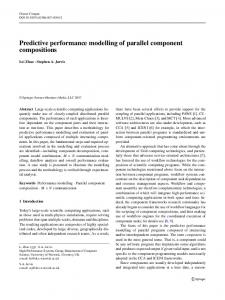
4.2 Performance evaluation If not otherwise specified, the packet size is constant in all the experiments and the transport layer payload is equal to 1448 bytes. The header at the IP layer is 20 bytes long, while the header at the TCP layer is 32 bytes long, because the header contained the optional timestamp field. This corresponds to generate MTU-sized IP packets. In the following we will show results obtained using W = 16 MSS. We have also carried out tests investigating the impact of the size of the TCP receiver’s advertised window and we obtained similar results that are not reported here for space limitations. In Section 3.2.1 we demonstrated using simulations, that

5000

Nu=0, Nd=n

4000 Throughput (Kbps)

0.45

Nu=1, Nd=n

3000 Nu=n, Nd=n 2000 Nu=n, Nd=1

1000 analysis experiments

0 1

2

3

4

5

6

n

Figure 3: Comparison of model predictions with measured ρD . our model is capable of precisely describing the network behaviour from the perspective of the network backlog distribution. The following experimental results validate the correctness of our model to compute the TCP data transfer throughput in a large variety of network configurations. To this end, the curves plotted in Figure 3 and Figure 4 compare the throughput performance measured during the experiments with the model predictions for different mix of TCP

5000 4000 Throughput (Kbps)

that could be frequently in idle state, without data (or acknowledgment) packets to transmit, while the access point stores most of the traffic generated by the TCP connections. As a consequence, the TCP traffic generates a very low contention in the WLAN. The results of this paper provide a useful insight in the behaviour of TCP data flows in 802.11-based WLANs. In addition, our proposed model could be the analytical basis for optimizing the network capacity and improving the system capabilities. To this end we are currently exploring several possible extensions/enhancements of our modelling framework, such as to integrate in the model short-lived TCP connections, UDP flows and prioritization mechanisms.

Nu=n, Nd=0 Nu=n, Nd=1

3000 Nu=n, Nd=n 2000 Nu=1, Nd=n

1000 analysis experiments

0 1

2

6. REFERENCES 3

4

5

6

n

Figure 4: Comparison of model predictions with measured ρU . downstream and upstream flows. More precisely, Figure 3 shows the throughput of downlink connections, while Figure 4 shows the throughput of TCP uplink connections. From the graphs, we can note that our model provides a very good correspondence between the analysis and the measured throughputs in all the considered configurations. The results plotted in Figures 3 and 4 also indicate that when there are not buffer overflows at the AP’s output queue the TCP flows fairly share the 802.11 channel bandwidth, irrespective of the number of wireless stations that are TCP receivers or TCP senders. In addition, the aggregate TCP throughput is almost constant and independent of the number of open TCP flows. The reason is that the interactions between the MAC protocol and the TCP flow control algorithm limit the average network contention level to a few stations. Consequently, the impact of collisions on the throughput performance is negligible and independent of the number of wireless stations in the WLAN. This is in contrast with the typical behaviour of a saturated network, in which the collision probability increases by increasing the number of wireless stations. These findings further reinforce our claim that the accurate modelling of TCP in 802.11-based WLANs cannot be carried out using saturation analysis.

5.

CONCLUSIONS

In this paper we investigated the throughput performance of persistent TCP-controlled download and upload data transfers in typical 802.11-based WLAN installations through analysis, simulations and experimentation. Based on a large set of experiments conducted in a real network, we found that: i) using default settings for the capacity of devices’ output queues provides a fair throughput ratio between upload and download connections; and ii) the total TCP throughput does not degrade when increasing the number of wireless stations. To explain the observed TCP behaviours we developed an analytical model of the interactions between the MAC protocol and the TCP flow control algorithm. The developed analysis is used to derive the network backlog distribution and to characterize the buffers’ occupancy in the presence of persistent TCP upload and download connections. By embedding the network backlog distribution in the MAC protocol modelling we were able to precisely describe the TCP evolution and to accurately evaluate the TCP throughput performance. Our analytical results show that the interaction between the contention avoidance part of the 802.11 MAC protocol and the closed-loop nature of TCP induces a bursty TCP behaviour with the TCP senders (or the TCP receivers)

[1] A. Abouzeid, S. Roy, and M. Azizoglou. Comprehensive Performance Analysis of a TCP Session Over a Wireless Fading Link With Queueing. IEEE Trans. Wireless Commun., 2(2):344–356, March 2003. [2] F. Alizadeh-Shabdiz and S. Subramaniam. A Finite Load Analytical Model for IEEE 802.11 Distributed Coordination Fucntion MAC. In Proc. ACM WiOpt’03, Sophia-Antipolis, France, March 3–5 2003. [3] E. Altman, K. Avrachenkov, and C. Barakat. A Stochastic Model of TCP/IP With Stationary Random Losses. IEEE/ACM Trans. Networking, 13(2):356–369, April 2005. [4] G. Bianchi. Performance Analysis of the IEEE 802.11 Distributed Coordination Function. IEEE J. Select. Areas Commun., 18(9):1787–1800, March 2000. [5] R. Bruno, M. Conti, and E. Gregori. Analytical Modeling of TCP Clients in Wi-Fi Hot Spot Networks. In Proc. IFIP-TC6 Networking Conference, pages 626–637, Athens, Greece, May 9–14 2004. [6] R. Bruno, M. Conti, and E. Gregori. Modeling TCP Throughput over Wireless LANs. In Proc. IMACS World Congress on Scientific Computation, Applied Mathematics and Simulation, Paris, France, July 11–15 2005. [7] R. Bruno, M. Conti, and E. Gregori. Performance Modelling and Measurements of TCP Transfer Throughput in 802.11-based WLANs. Technical Report 02/2006, IIT - CNR Pisa, April 2006. [Online]: http://bruno1.iit.cnr.it/∼bruno/publications.html. [8] F. Cal´ı, M. Conti, and E. Gregori. Dynamic Tuning of the IEEE 802.11 Protocol to Achieve a Theorethical Throughput Limit. IEEE/ACM Trans. Networking, 8(6):785–799, 2000. [9] G. Cantieni, Q. Ni, C. Barakat, and T. Turletti. Performance analysis of IEEE 802.11 DCF under finite load traffic. Elsevier Computer Commun. Journal, 28:1095–1109, June 2005. [10] K. Duffy, D. Malone, and D. Leith. Modeling the 802.11 Distributed Coordinated Function in Non-Saturated Conditions. IEEE Commun. Lett., 9(8):715–717, August 2005. [11] M. Garetto, R. Lo Cigno, M. Meo, and M. Marsan. Closed Queueing Network Models of Interacting Long-Lived TCP Flows. IEEE/ACM Trans. Networking, 12(2):300–311, April 2004. [12] D. Heyman and M. Sobel. Stochastic Modles in Operations Research, volume 1. McGraw-Hill, New York, NY, 2001. [13] IEEE 802.11. The Working Group for WLAN Standards, April 2006. http://grouper.ieee.org/groups/802/11/. [14] A. Kumar, E. Altman, D. Miorandi, and M. Goyal. New Insights from a Fixed Point Analysis of Single Cell IEEE 802.11 WLANs. In Proc. IEEE INFOCOM 2005, volume 3, pages 1550–1561, Miami, Florida, USA, March 13–17 2005. [15] D. Miorandi, A. Kherani, and E. Altman. A Queueing Model for HTTP Traffic over IEEE 802.11 WLANs. Elsevier Computer Networks Journal, 50(1):63–79, January 2006. [16] NLANR/DAST. Iperf Version 2.0.2, May 3 2005. http://dast.nlanr.net/Projects/Iperf/. [17] J. Padhye, V. Firoiu, D. Towsley, and J. Kurose. Modeling TCP Throughput: a Simple Model and its Empirical Validation. IEEE/ACM Trans. Networking, 8(2):133–145, April 2000. [18] S. Pilosof, R. Ramjee, D. Raz, Y. Shavitt, and P. Sinha. Understanding TCP fairness over Wireless LAN. In Proc. IEEE INFOCOM 2003, volume 2, pages 863–872, San Francisco, USA, March 30– April 3 2003. [19] W. Stevens. TCP/IP Illustrated, Volume 1: The Protocols. Addison-Wesley, New York, NY, December 1993. [20] Y. Tay and K. Chua. A Capacity Analysis for the IEEE 802.11 MAC Protocol. Wireless Networks, 7:159–171, 2001. [21] O. Tickoo and B. Sikdar. A queueing model for finite load IEEE 802.11 random access. In Proc. IEEE International Conference on Communications (ICC), volume 1, pages 175–179, Miami, Florida, USA, June 13–17 2004.