cycle to allow virtual prototyping and testing of products prior to the physical ... the results of a finite element simulation of a grinding process, a simple but.
Performance Models of Interactive, Immersive Visualization for Scienti c Applications Valerie E. Taylor
EECS Department, Northwestern University Evanston, Illinois USA
Rick Stevens
Thomas Can eld
MCS Department, Argonne National Laboratory Argonne, Illinois USA
Abstract
In this paper we develop a performance model for analyzing the endto-end lag in a combined supercomputer/virtual environment. We rst present a general model and then use this model to analyze the lag of an interactive, immersive visualization of a scienti c application. This application consists of a nite element simulation executed on an IBM SP-2 parallel supercomputer and the results displayed in real-time in the CAVE Automatic Virtual Environment. Our model decouples the viewpoint lag (not involving the simulation) from the interaction lag (using the results of the simulations). This model allows one to understand the relative contributions to end-to-end lag of the following components: rendering, tracking, network latency, simulation time, and various types of synchronization lags. The results of the study indicate that the rendering and network latency are the major contributors of the end-to-end lag.
1
1 Introduction Interactive, immersive visualization allows observers to move freely about computer generated 3D objects and to explore new environments. This technology can be used to extend our perception and understanding of the real world by enabling observation of events that take place in spaces that are remote, protracted or dilated in time, hazardous, or too small or large to view intricate details. The 3D environment can be a distortion of reality projected on a physical framework that enables the display of non-visual, physical information, such as temperature, velocity, electric and magnetic elds, and stresses and strains. In engineering, this technology may be incorporated into the product design cycle to allow virtual prototyping and testing of products prior to the physical construction. Hence, interactive, immersive 3D visualization is an important medium for scienti c applications. An interactive, immersive visualization of scienti c simulations involves four major components: the graphics system, the display system, the simulation system, and the communications between the various components. The graphics system performs the calculations for the rendering of the objects used in the display. These calculations are computationally intensive and often require high-performance computers, especially for volume reconstruction. The display system consists of the screen, projectors, interactive devices, and tracking sensors. The user interacts with the 3D objects via devices such as a head tracker or hand-held wand (similar to a mouse). The simulation system performs the calculations for the analysis of the scienti c phenomenon. Again high-performance computers, often parallel systems, are required to reduce the execution time of the simulation. The last component consists of the connections used to communicate information between the user (via the display) and the graphics system and between the graphics and simulation systems. A critical issue to be addressed is how to reduce the end-to-end lag time, i.e., the delay between a user action and the display of the result of that action. Liu et. al. [9] found lag time to be equally important as frame rate for immersive displays. Lag has been studied in the context of teleoperated machines, head-mounted displays, and telepresence systems [9, 16]. The goal of this paper is to extend these models and techniques for lag analysis to include integrated supercomputer applications with interactive, immersive virtual interfaces. The addition of supercomputer simulations into the virtual environment increases the complexity of the models. Hence, these models are important for understanding the impact of the various system components on the lag time. We conduct an extensive case study of a visualization system to display the results of a nite element simulation of a grinding process, a simple but widely used manufacturing task. The display system consists of a CAVE (Cave Automatic Virtual Environment) [11], an interactive immersive 3D system. We have instrumented all major processes in the system and have developed a performance model that allows us to understand the relative contributions to end-to-end lag of rendering, tracking, local network connections to the supercomputer, supercomputer simulation, and various types of synchronization lags. The concepts presented in this paper can be extended easily to other scienti c applications, using both local and remote supercomputers. Our model decouples the viewpoint lag (not involving the simulation) from
the interaction lag (using the simulation results). Our analysis indicate that the major component of viewpoint lag is the rendering lag. For the interaction lag, majority of the time is comprised of rendering and network lags. The remainder of the paper is organized as follows. In Section 2 we discuss previous work, followed by the details of the visualization environment available at Argonne National Laboratory (the site where this study was conducted) in Section 3. We present our general model for end-to-end lag in Section 4. The ndings of the case study are given in Section 5. We discuss methods for reducing the lag in Section 6 and summarize the paper in Section 7.
2 Previous Work In [16] Wloka presents a thorough analysis of lag time in multiprocessor virtual reality systems. The focus is on the viewpoint lag. He identi es the various sources of lag time: input device lag | time required to obtain position and angle measurements of input device, application lag | application-speci c processing of input device mechanism, rendering lag | time to render the data and display it, synchronization lag | total time the sample is waiting between processing stages, and frame-rate induced lag | the time between changes in the display. In Wloka's system, the application-speci c processing is directly dependent on one user input device. In contrast, we analyze an existing system for which the user has two input devices, the head tracker (which a�ects the viewpoint and interaction lags) and the wand (which a�ects the interaction lag). Methods for reducing the lag in our system must consider the relationship between the two lags; a reduction in lag for one input device may result in an increase in lag for a second input device. Further, our system includes a parallel machine and a shared-memory multiprocessor system connected via a network. Therefore, we consider two additional sources of lag: the network lag and simulation lag. In [10] Mine characterizes the relative performance of various tracking technologies, which include two magnetic trackers from Ascension Technology Corporation and two from Polhemus Incorporated. This characterization is considered in the context of reducing end-to-end delay in head-mounted systems. The focus, however, is on the tracking lag only; no attention is given to the other sources of lag. In contrast, we consider all the sources of lag in our existing system. Methods for reducing lag is an active area of research. Such methods include prediction [8, 3, 1], time-critical computing [4, 5, 15], and use of parallelism. Prediction methods use extrapolation to reduce tracker lag by predicting future input data based upon past data. These methods require that the other components of lag have constant lag times. This is generally not the case, especially for systems including scienti c simulations executed on supercomputers. Time-critical computing trades computation time for computation accuracy, which is not advisable for directly reducing lag. The use of parallelism reduces the lag by increasing the computing resources used for the computations. In this paper we consider the use of parallelism with the simulation and graphics. We also discuss the bene ts of reduction in scene complexity for reducing lag.
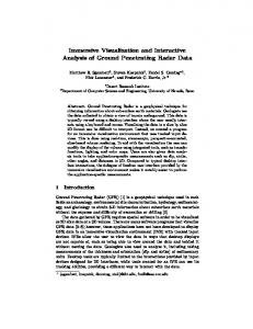
Figure 1: Supercomputing/Visualization environment.
3 Visualization Environment
The interactive, immersive simulation environment at Argonne National Laboratory consists of a 128-node IBM SP-2 system, an SGI Onyx, network connections between the SGI Onyx and IBM SP-2, and a CAVE as illustrated in Figure 1 . Currently, the network connection can be con gured to be an ATM OC-3c, NSC HIPPI switch, or Ethernet. Because of the focus on performance, we provide details of the various components of the environment.
3.1 Display Component
The CAVE, the display component, creates a large eld of view by projecting images onto two walls and the oor of a ten-foot cube. Infrared emitters are synchronized to the projectors to provide a stereo sync for the Crystaleyes LCD glasses worn by each user. Stereo cues are provided by displaying sequentially images of the left-eye view followed by the right-eye view. Tracking is provided by an Ascension Flock of Birds tracking system with two input modules. One sensor is used to track the head movements, and the other is for the handheld wand. The sensor on the wand is slaved to the head sensor, which is connected via a serial line to the SGI Onyx. The wand also has three buttons and a joystick for interacting with the virtual world. The wand buttons and joystick are interfaced to the SGI Onyx via an IBM PC, which provides A/D conversion, debounce, and calibration. In the CAVE, the scientist is e�ectively immersed in the phenomenon under study and provides input to the simulation or experiment via the wand. In addition, other observers can passively share the virtual reality experience by wearing the LCD glasses. Ascension Flock of Birds sensors are used to generate the position and angle of the head unit and the wand. These sensors can perform updates at the rate
of 10 to 144 measurements per second [2]. The existing system is con gured to operate in the range of 100 measurements per second. The buttons on the wand are sampled by an IBM PC at the rate of 100 Hz.
3.2 Graphics Component
The SGI Onyx is a shared-memory multiprocessor system with an extensive graphics subsystem. Our system has 128 MB RAM, 10 GB disk, four R4400 processors and three RealityEngine2 graphics pipelines; the system runs Irix 5.3 and AFS. Each RealityEngine2 has a geometry engine consisting of Intel i860 microprocessors, a display generator, and 4 MB raster memory [13]. The Onyx is used to drive the virtual environment interface. Each graphics pipe is connected to an Electrohome Marque 8000 high-resolution projector, which projects a high-resolution image onto the screens of the CAVE. The projectors are running at 96 Hz frame rate in stereo mode. All of the CAVE code is executed on the SGI Onyx, using all four R4400 processors. The code consists of ve processes: a main, three rendering, and one tracker. The main routine is responsible for sending and receiving data to and from the simulation. The rendering loops perform the calculations for the surface graphics, and the tracker loop obtains the interactive commands. The three rendering processes, corresponding to the two walls and the oor, each run on a dedicated R4400 processor; these processes synchronize at the end of the rendering calculations for each frame. The tracker and main processes time share the fourth processor. The code is explained further in Section 4.
3.3 Simulation Component
The simulation component consists of a large-scale, 128-processor IBM SP-2 supercomputer with a high-performance I/O environment. This system is used for general-purpose parallel supercomputing. Each SP node has 128 MB RAM, 1 GB local disk and is connected to other processors via a TB-2 high-speed interface to the IBM vulcan switch. Some of the processors in this system have been equipped with ATM, HIPPI, and Ethernet interfaces. The IBM system is also interfaced to 220 GB of high speed RAID disk and connected to an Ampex DST-800 automated tape library. The I/O system of the IBM SP-2 will eventually be used for CAVE recording and playback experiments, but that work is beyond the scope of this paper. Simulations are executed on the SP-2 using a scheduler developed at Argonne and can be run in batch or interactive mode. For e�cient access, the processors used in the simulation with the CAVE cannot be scheduled by other users.
3.4 Interconnections
A user controls the eld of view with the head tracker and simulation parameters with the wand. As discussed previously, the IBM PC and Flock of Birds tracking system are connected to two Onyx serial ports as illustrated in Figure 1. The IBM SP-2 and SGI Onyx communicate via an ATM OC-3c, NSC HIPPI switch, or Ethernet. The ATM network uses a Fore Systems switch and both 100 Mbps and 155 Mbps cards. The HIPPI interface is a 800 Mbps network that connects via a Network Systems Corporation's HIPPI switch. The
Ethernet provides a 10 Mbps connection. The IBM SP-2 and the SGI Onyx are within the same building, allowing us to use LAN networking technology for these experiments. One of our long-term goals is to use multiple supercomputers and multiple CAVEs and derivatives (like ImmersaDesks and HMDs) for wide area collaborative use.
4 Performance Model Recall from Section 1 that the metric that we are attempting to minimize is the lag time of the user interaction. Given two input devices, we consider two classi cations of interactions: � movement of the head tracker: this type of interaction causes a change to the eld of view; the data sent to the simulation process is not modi ed | the lag is de ned as view Q
movement and clicking of wand buttons: this type of interaction causes modi cations to the simulation process, for which the results causes a change to the graphics (dictated by the meaning of the wand buttons) | the lag is de ned as interact The operations that are executed based upon a user interaction are the following: 1. The sensors generate the position and rotation of the header tracker and wand; the personal computer records the position of the wand buttons ( track ) [input device lag] �
Q
T
2. The wand data (read by the rendering process) is sent to the simulation process ( write) [network write lag] T
3. The simulation process uses this data to update the analysis ( sim ) [simulation lag] T
4. The graphics process reads the newly generated simulation results ( read ) [network read lag] T
5. The graphics process uses the data from the simulation process and the tracker to render a new image ( render ) [rendering lag] In addition to the above lags there is also synchronization lag as described previously. We consider four sources of synchronization lag: (1) sync(TR): the time from when the tracker measurement is available until the data is read by one of the rendering processes, (2) sync(RS ): the time from when the rendering process has read the updated wand values until the values are available for writing to the simulation process, (3) sync(SR): the time from when the data is available from the simulation process until used by the rendering process, and (4) sync(F ) the time from when the data is available in the frame bu�er and the image is available on the screen. T
T
T
T
T
Figure 2: Components of lag time for view and interact. Q
Q
Given the above sequence of operations, the following equations represent the lag time for the head tracker ( view) and the wand ( interact): (1) view = track + sync(TR) + render + sync(F ) interact = track + sync(TR) + sync(RS ) + write + sim + read + (2) sync(SR) + render + sync(F ) The derivation of these equations is discussed in the following section. Q
Q
Q
Q
T
T
T
T
T
T
T
4.1 Lag Sources
T
T
T
T
T
T
In Figure 2, we provide a detailed diagram of the various lag terms and their relations to the lag time equations. The model assumes an asynchronous process implementation of the system (i.e., each major process of the system is running asynchronously). This assumption is consistent with the actual implementation of the visualization environment. The diagram consists of six major processes. Recall from Section 3.2 that the CAVE code entails ve processes: one main process, three rendering processes, and one tracker process. The sixth process consists of the simulation, which may be executing on one or more processors of the IBM SP-2. In this paper, we consider the simulation to be one process. More advanced models may support the simulation as a number of processes that may be able to communicate intermediate data to the rendering process or stagger communication to reduce network latency. The main process runs on the Onyx and is responsible for initiating the rendering processes (this is done only once) and communicating with the simulation process. Hence this process has three states: writing data via the network
to the SP-2, reading data via the network from the SP-2, and copying the simulation data to the SGI shared memory to be used by the rendering processes. The time devoted to the memory copy is negligible and therefore not included in the model. The simulation process consists of three states: reading from the network from the main process, processing the simulation update, or writing data to the network for the main process. Any wait time incurred with the network is considered part of the corresponding read or write time. There are three rendering processes used for the displays on the two walls and the oor of the CAVE. These processes are indicated in the diagram as Render0, Render1, and Render2. These processes are essentially identical with the exception of Render0 process, which reads the tracking data from the tracking process and makes it available to the other rendering process. Only one rendering process performs this task to insure that all three rendering processes are performing calculations in response to the same tracker data. The rendering processes use the tracking and simulation data to render the six images displayed in the CAVE; they synchronize at the end of each frame and dump their bu�ers. The tracker process is responsible for continuously reading the tracking information from the serial SGI ports, scaling the data, and writing the data into a region of memory for reference by Render0. The tracker process is also responsible for initialization of the tracker and wand controls. The tracker process, like the other processes, operates asynchronously, reading tracker data as fast as the tracking system can produce it.
4.2 Lag Equations
The diagram in Figure 2 illustrates all the sources of lag that are used in our model. Assuming a wand and tracker event occurs as indicated in the diagram, we can trace the lag times that result in a scene update due to a head event (indicated in the diagram) and a scene update due to a wand event (indicated in the diagram). When a head tracker event occurs, the tracker process reads the values from the Flock of Birds ports, perform the calibration, and places these values in shared memory. The time to execute these operations is given by tracker in Equations (1) and (2). Typically, the tracker process is sampling the sensors faster that the rendering process can render a new display. Only the last sample obtained prior to the start of a new rendering cycle is read by the rendering process. Hence, the average \wait time" or synchronization lag is half the average tracker update time. This time corresponds to sync(TR) in the equations. The head tracker sample, read by Render0 process, is used by the three rendering processes to render a new image. This corresponds to render in the equation. When the new image data is available, it may not be displayed immediately. There is some wait time due to the frame rate and the scan rate of the projectors. The average of this synchronization time is half the frame and scan times per eye for stereo; this time is given by sync(F ) in the equations. Lastly, we get the scene update from the head tracker event. The summation of these four terms compose the viewpoint lag or view . When a wand tracker event occurs, the sensors are again sampled by the tracker process and read by Render0 process. This task corresponds to tracker and sync(TR) as described above. At this point, the analysis takes a di�erent T
T
T
T
Q
T
T
path from that taken with the viewpoint lag. Once the wand position has been read by Render0 process, it is used by the main process to forward to the simulation process. This wand data may not be read immediately by the main process. The average time that this data \waits" to be used is equal to half the time of the main process. This synchronization time corresponds to sync(RS ) in Equation (2). The main process sends these wand values to the simulation process to be used for updates to the simulation analysis. These values are sent across the network connecting the SGI to the IBM SP-2. This time corresponds to write. The simulation time is denoted by the term sim . The updated simulation values are then sent to the main process, corresponding to a read by the main process. This time is denoted by the term read . After the data is read by the main process, it may not be used immediately by the rendering processes. The average of this \wait" time is equal to half the average of the rendering time; this synchronization time is denoted as sync(SR). Once the values have been read by the rendering processes, a new image is rendered and displayed corresponding to render + sync(F ) . The summation of these nine terms compose the interaction lag or interact. T
T
T
T
T
T
T
Q
5 Case Study: Grinding Process
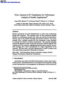
The problem used in this study is a computer simulation of a grinding process, which is commonly used in manufacturing environments. A picture of the virtual grinder is given in Figure 3. An operator is immersed in a machine room and can perform the task of grinding a part with a wheel by controlling the motion of the three axes of a table with the wand. When the wheel is in contact with the part on the table, heat is generated as a result of the grinding motion. Internal stress and ow of heat are produced in the part, wheel, and table. The temperature and stress for a simple system are computed in real time on the IBM SP-2; the simulations involve multibody dynamics and nite element analysis. The results are selectively displayed on the various components. Materials ablated by the grinding are ejected as small particles and displayed as sparks. This prototype is indicative of larger systems used to analyze complex mechanical systems, including the detection of contacting surfaces, friction at the interfaces, large rigid body motions, and thermal-mechanical analysis with nite elements. The virtual grinder is fairly simple in that it has 433 elements and 788 nodes. The analysis involved in this simple problem is representative of more complex structures such as an automotive disk brake with approximately 4000 elements and 6000 nodes just to model the pads and rotor. Because of the simplicity of our example, the simulation of the grinding process is executed on one processor of the IBM SP-2. Hence the focus is on the analysis of the simulation with CAVE; we do not focus on the decomposition methods or interprocessor communication of the parallel machine. These issues, however, are discussed brie y in Section 6.3.
5.1 Timing Relationships
The CAVE library and the application code were instrumented using the Pablo system [12] and some SGI timing routines. The average time for each lag source
Figure 3: Virtual grinder.
Table 1: Various lag values for the base case. Mean Std. Dev. % view % interact
Lag
(ms)
30.0 15.0 208.0 99.0 0.102 21.8 197.0 104.2 15.0
track sync(TR) Trender Tsync(RS ) Twrite Tsim Tread Tsync(SR) Tsync(F ) T T
(ms)
8.8 | 0.069 | 0.048 1.2 65.0 | |
Q
Q
11.19 5.60 77.61 NA NA NA NA NA 5.60
4.34 2.17 30.14 14.35 0.01 3.16 28.55 15.1 2.17
is given in Table 1. The timings along with the standard deviations are based upon a sample space of 300-400 data points. The values with no corresponding standard deviations correspond to the sources of synchronization lag, which are derived from other values. The total lag time for view = 268 0 ms and interact = 690 0 ms. As a point of reference, Liu et. al. [9] conducted experiments on a telemanipulation system and found the allowable lag time to be 100 ms and 1000 ms (1s) for inexperienced and experienced users, respectively. The sync(F ) value is based upon a frame rate of 48 frames per second per eye and an average scan rate of 120 Hz for the Marquee 8000 projectors. The average of this synchronization lag is equal to one half of the frame-induce time. The system con guration consisted of a Ethernet connection between the SGI Onyx and IBM SP-2. The values indicate that the rendering time is the major lag component for viewpoint lag, view , comprising 77.61% of the lag time. For interact, the rendering and read network times are the major lag components, together comprising 58.69% of the lag time. For the case involving a very complex simulation, the pro le of interact will change with the possibility of the simulation time also being a major component of the lag time; the view pro le would remain the same. Q
Q
:
:
T
Q
Q
Q
Q
6 Lag-Reducing Methods
In this section we consider methods for reducing the end-to-end lag. We focus on the rendering, simulation, and network lags, which can be major factors a�ecting the end-to-end lag as discussed in the previous section. In particular we focus on scene complexity, networks, and parallelism.
6.1 Scene Complexity
The rendering lag is a function of the scene complexity and the geometry transformations. This scene consists of essential objects a�ected by the simulation and the background used to give the scientist the illusion of being in the remote environment. For the grinder application, the essential objects are the table, part, and wheel. The image of the tool shop creates an illusion of being in a
Table 2: Various lag values for the reduction in scene complexity. Lag Mean Std. Dev. % view % interact track sync(TR) Trender Tsync(RS ) Twrite Tsim Tread Tsync(SR) Tsync(F ) T T
(ms)
Q
(ms)
30.0 15.0 67.5 99.0 0.102 21.8 197.0 34.0 15.0
8.8 | 8.8 | 0.048 1.2 65.0 | |
Q
23.53 11.76 47.37 NA NA NA NA NA 11.76
6.26 3.13 14.09 20.67 0.02 4.55 41.13 7.10 3.13
manufacturing setting. The rendering lag can be reduced by reducing the complexity of the background without sacri cing the interface to the simulation. We conducted an experiment to determine how much reduction can occur when reducing the scene complexity. In particular, we eliminated all the rendering code associated with the background, the image of the machine shop, and extracted the new times of each of the sources of lag. The results are given in Table 2. The total time for view = 127 5 ms and interact = 479 0 ms. The results indicate that the rendering time is reduced by a factor of one third { 208 ms to 67.5 ms. This reduction results in a interact reduction by a factor of two thirds { 690 ms to 479 ms, and a view reduction by a factor of one half { 268 ms to 127.5 ms. Hence reduction in scene complexity had a major impact on the lag time for the grinder application. The read network time becomes the major factor with interact. Q
:
Q
:
Q
Q
Q
6.2 Network Latency
The current con guration of the supercomputing/virtual environment consists uses a local Ethernet connection. The use of HIPPI only connections or ATM only connections would reduce the time needed for read and write . The network connections become very important if the supercomputing involved is located at a remote site, involving WAN connections. For this case the network latency can dominate the interaction lag. Latency-hiding techniques must be used to overcome this lag. This can be achieved by overlapping the simulation computation with the shipping of the generated data. The network would be time multiplexed between the simulation processors such that it is always busy shipping data. T
6.3 Parallelism
T
Further parallelism can be exploited with the rendering algorithms as well as the simulation. Parallel graphics algorithms is a very active area of research. Parallelism is exploited in the CAVE environment by spawning o� processes for the tracking systems and the three rendering processes. Further parallelism
can be exploited within each rendering process in terms of the di�erent objects involved in the display. Much work has been done with parallel nite element analysis. This work involves exploiting the data parallelism available in the problem. For this environment, the network connection must also be considered. The decomposition method must incorporate strategies for keeping the network connection to the graphics process as busy as possible, as discussed above. The network lag can by a major contributor of the interaction lag as illustrated by the preceding section in which read was the major component of the interaction lag for the display with no texturing. T
7 Summary Lag has been often studied in the context of teleoperated machines, headmounted displays, and telepresence systems [9, 16]. In this paper we extended these models and techniques for lag analysis to those suitable for analysis of integrated supercomputer applications with interactive, immersive virtual interfaces. This extension consisted of the addition of two additional sources of end-to-end lag, network time and simulation time. We provided the framework of a performance model to provide insight on the major contributions of lag time for supercomputing/virtual environment. We conducted an extensive case study of a supercomputing/virtual system used to display the results of a nite element simulation of a grinding process, a simple but widely used manufacturing task. The results indicated that the rendering time is the major component for viewpoint lag, view, comprising 55.61% of the lag time. For interact, the rendering and read network times are the major lag components, together comprising 58.69% of the lag time. For the case when of a very complex simulation, the pro le of interact will change with the simulation time also being a major component of the lag time; the view pro le would remain the same. We also discussed some methods to reduce the end-to-end lag for a supercomputing/virtual system. We considered scene complexity, parallelism, and network latency. We conducted an experiment to measure the impact on lag time from reducing the scene complexity. The results indicated that the rendering time is reduced by a factor of one third { 208 ms to 67.5 ms. This reduction results in a interact reduction by a factor of two thirds { 690 ms to 479 ms, and a view reduction by a factor of one half { 268 ms to 127.5 ms. Hence reduction in scene complexity had a major impact on the lag time for the grinder applications. Q
Q
Q
Q
Q
Q
Acknowledgments The authors acknowledge Chris Stau�er for the time devoted to collecting some of the data used in this paper and Micheal Papka, Terry Disz, Shannon Bradshaw, and William Nickless for the hours of discussions about the CAVE. The rst author was supported by a National Science Foundation Young Investigator Award, under grant CCR{9357781. The second and third authors were
supported by the O�ce of Scienti c Computing, U.S. Department of Energy, under Contract W-31-109-Eng-38.
References
[1] Deering M. High Resolution Virtual Reality. Computer Graphics 1992; 26:195-202 [2] The Flock of Birds Installation and Operation Guide, Ascension Technology Corporation, 1994 [3] Friedmann M, Starner T, Pentland A. Device Synchronization Using an Optimal Linear Filter. Computer Graphics 1992; 25:57-62 [4] Funkhouser T, Sequin C H. Adaptive Display Algorithm for Interactive Frame During Visualization of Complex Virtual Environments. Computer Graphics 1993; 27:247-254 [5] Holloway R L. Viper: A Quasi-real-time Virtual Worlds Application. Technical Report TR92-0004, University of North Carolina at Chapel Hill, 1991 [6] Hughes T. The Finite Element Method, Prentice-Hall, Inc., Englewood Cli�s, NJ, 1987 [7] Jones M, Plassmann P. Solution of Large, Sparse Systems of Linear Equations in Massively Parallel Applications. In: Proceedings of Supercomputing, 1992 [8] Liang J, Shaw C, Green M. On Temporal-Spatial Realism in the Virtual Reality Environment. In: Proceedings of the 1991 User Interface Software Technology, 1991, pp 19-25 [9] Liu A, Tharp G, French L, Lai S, Stark L. Some of What One Needs to Know about Using Head-Mounted Displays to Improve Teleoperator Performance. IEEE Transactions on Robotics and Automation 1993; 9:638648 [10] Mine M R. Characterization of End-to-End Delays in Head-Mounted Display System. Technical Report TR93-001, University of North Carolina at Chapel Hill, 1993 [11] Cruz-Neira C, Sandin D J, DeFanti T. Surround-Screen Projection-Based Virtual Reality: The Design and Implementation of the CAVE. In: Proceedings of SIGGRAPH, 1993, pp 135-142 [12] Noe R. Pablo Instrumentation Environment User's Guide. University of Illinois at Urbana-Champaign, Department of Computer Science, 1994 [13] Silicon Graphics Onyx Installation Guide. Document Number 108-7042010. [14] Smith B, Gropp W. Scalable, Extensible, and Portable Numerical Libraries. In: Proceedings of Scalable Parallel Libraries Conference,1993, pp 87-93
[15] Wloka M. Time-critical Graphics. Technical Report CS-93-50. Brown University, Department of Computer Science, 1993 [16] Wloka M. Lag in Multiprocessor Virtual Reality. Presence 1995; 4:50-63