15 min in a Data General or VAX computer for a 32 X 32 pixel object if it is successful, .... to increase, one is not likely to get stuck in the nearest local minimum. ..... struction for astronomy," in Image Recovery: Theory and Ap- plication, H. Stark ...
30
J. Opt. Soc. Am. A/Vol. 5, No. 1/January 1988
Nieto-Vesperinas et al.
Performance of a simulated-annealing algorithm for phase retrieval M. Nieto-Vesperinas and R. Navarro Instituto de Optica, Consejo Superior de Investigaciones Cientifficas,Serrano,121, 28006 Madrid, Spain
F. J.Fuentes Instituto de Astrofisica de Canarias, 38071 La Laguna, Tenerife, Spain Received March 10, 1987; accepted June 10, 1987 We report computer observations on the performance of an improved version of a simulated-annealing algorithm that was used before for the problem of phase retrieval. According to the results, we propose to use this method in conjunction with the algorithm of Fienup [Opt. Lett. 3, 27 (1978); Opt. Eng. 18, 529 (1979); Appl. Opt. 21, 2758 (1982). The full power of the simulated-annealing algorithm with large arrays appears to be limited by present-day computers rather than by its numerical performance, but we believe that this combination may constitute an efficient method for phase retrieval.
1. INTRODUCTION The question of phase retrieval often appears in optics and other areas of physics such as x-ray diffraction, scattering, and astronomy. We shall deal with this subject for the case in which one intensity measurement is available in the Fourier domain. At present it is widely accepted that although phase reconstruction is nonunique in one dimension, there is a high probability that it is unique in two or more dimensions', 2 [although a certain amount of noise (uncertainty) in the data could increase the chance that they were approximately compatible with those of a nonunique situation]. Let g(x, y) be a function representing a two-dimensional object with finite support (i.e., zero outside a certain domain), and let G(u, v) = G(u, u)iexp[i(u, v)] be its Fourier transform; the phase problem consists of finding the phase q5(u, v) from the known modulus !G(u, v)I and certain restrictions on the object g(x, y). Here, we shall consider the restrictions to be nonnegativity and finite support. In the (x, y) space, with digital methods, assuming a discrete model, this is equivalent to solving the set of nonlinear equations described by M
Qij
M
I gmngm+i-M,n+j-Mt
m=1 n=1
1
m 0, then the change is accepted with a
probability exp(-AF/T). To do this, we take a number n from a sequence of random numbers uniformly distributed in the interval (0, 1). If n is less than exp(-AF/T), then the change is accepted, and one starts with the next pixel. If n is greater than or equal to exp(-AF/T), then the change is not
accepted, and one starts with the next pixel. All pixels of the object are scanned in this way for as many cycles as necessary until equilibrium is reached, i.e., when on the average the number of trials increasing F equals the number of trials decreasing F. T is then lowered, and one starts the procedure again. The larger T is, the higher the probability is of accepting a change raising F. Thus, since F is allowed to increase, one is not likely to get stuck in the nearest local minimum. Eventually, when one is near the end of the algorithm, at very low values of T, only changes lowering F
are accepted. The scale of perturbation a must be chosen with care; if a is too large, F will oscillate highly or will yield forbidden
changes, and if a is too small, the reconstruction evolution will be too slow. The performance of the algorithm is en-
hanced if a is allowed to decrease as T - 0 according to a certain schedule. The fast computation of the autocorrelation function of the corresponding iteration with a perturbed pixel is a nontrivial matter. The most efficient way that we have found is to follow the scheme Q(m+l)(xy)
=
J
7)+ h6(
X [g(f)(lq + x,7y+ y) + h(
-
a, i
+x
-
-
VC
b)] a, y + y
-
b)]
= Q(m)(x, y) + hg()(a -x, b -y)
+ hg(m)(a
J
x, b +y) +h
25(x, Y).
(6)
In Eq. (6), Q(m+l)(x, y) is the autocorrelation function resulting from adding an amount h (-a < h a) to the pixel in (a, b) of the mth iteration of the objectg(m)(x, y), and 6(x, y) is the 3 function. A FORTRAN routine for the whole algorithm will be reported soon. 25 A block diagram of the algorithm is shown in Fig. 1. 3.
actions were done first; then we employed seven cycles, each containing one hundred hybrid input-output iterations followed by twenty error-reduction iterations. In all cases tested in this work, no further evolution of the reconstruction was observed by considerably increasing this number of cycles above seven or ten. In fact, 10 h of CPU time in a Data General computer and 2 h in a CDC Cyber computer were given to FA for a reconstruction from noiseless data of the objects of Plates 2(a) and 4(a). Neither reconstruction evolved from that of Plates 4(b) and 5(a), obtained with 28 min of CPU of FA, and the cost functions did not drop any further. This may be because of effects involved in the Fourier-transform operation, namely, the noisy and stripped features of Plates 4(b) and 5(a), respectively, seem to be due to biased phases acquired in the spectrum in the first iterations. No attempts were made to overcome stagnation by the methods of Refs. 15 and 16, however. For the SA algorithm, two annealing schedules were tested. One schedule features exponential decay, or T as T = exp[-h(n - 1)]TO in 50 steps n. is chosen such that To = 100 and T50 - 10-6; i.e., h = 0.37. The maximum number of cycles of object scan is set equal to 100. Equilibrium is considered reached when three consecutives times at the end of a cycle the number of accepted perturbations raising F differ from the number of perturbations lowering F (always accepted) to within 5%. The scale of perturbation a starts at a 1 and is modified at the end of each cycle according to the schedule ae, B{A + log FnP
Jdtdn[g()Q(,
COMPUTATIONAL RESULTS
Both the FA and the SA reconstructions were tested with 32 X 32 pixel objects. The FA was done by embedding the object in a 64 X 64 pixel window array to perform fast-
Fourier-transform operations. In all cases shown in this work the starting guess for both FA and SA was the one suggested by Fienup5 : take the autocorrelation data array Qij, save every other pixel in both dimensions and threshold
it to a value (we used 1O-4 with a maximum normalized to 1), and fill the results with random numbers. We usually obtain better performance of the algorithms by using this strategy than by starting with 32 X 32 pixel input arrays with random or constant values. FA was used with a feedback parameter g 0.7 in the hybrid input-output parts. Twenty error-reduction inter-
35
(7)
105; A equals the order of the initial cost function F (Fo thus A = 5). The exponent P establishes the change rate of a (P = 5 worked well), C is a number of chosen to make the
quotient no greater than 1 (we used C 16), and B scales the initial value a 0 to approximately 1 (we set B = 10). The other schedule tested, which produced similar results, contained the same number of steps of T as the first schedule but featured a linear decay of T; i.e., T,+1 = 0.75Th, and am = expf-(m - 1)], with the index m increasing one unit every
seven steps of variation in T. The chosen schedule therefore depends largely on the user. In any case, these choices of T and the scale of perturbation a are by no means exhaustive and must be considered merely concrete examples of performance of the SA algorithm in our case. A general rule, however, may be established, namely, that both the decay in T and the decay in c must be performed carefully and slowly. Otherwise, one is likely to be trapped in a local minimum of the cost function. All the examples to be shown in what follows took about 15-30 min of CPU time for FA and about 12-14 h of CPU time for SA in a Data General Eclipse MV 10000 computer. However, when the SA reconstruction was started with the FA result, the CPU time was reduced to about 6 h, provided that one tried to save perturbation scans near equilibrium. As mentioned before, with the astronomical objects, no improvement of the reconstructions was observed in the examples by letting FA run over comparable computing times. Since there are discussions among users on their relative successes in applying FA, we wish to report first a remarkable performance of this algorithm with a difficult synthetic
36
Nieto-Vesperinas et al.
J. Opt. Soc. Am. A/Vol. 5, No. 1/January 1988
(a)
(b)
Fig. 2. (a) Original object, which represents a 32 X 32 pixel lowpass-filtered version of object 5 of Ref. 21. (b) FA reconstruction from noiseless data.
pixel image of a galaxy recorded by astronomers of the Instituto Astrofisico de Canarias (IAC) with a charge-coupleddevice camera. We present it in color because of its large dynamic range. The autocorrelation and the power spectrum of this object are shown in Figs. 3(a) and 3(b), respectively. A logarithmic scale of gray levels has been used in Figs. 3(a) and 3(b); even so, the fainter outer details are not visible. FA reconstruction of this object from noisy data in the power spectrum with a S/N ratio of 10 is shown in Plate 2(b); the error is E = 1.7 X 10⁻². The error of the initial guess was E0 = 0.53. In terms of the cost function of Eq. (2), the reconstruction of Plate 2(b) has F = 10-2. The initial guess had a cost function F 0 = 69922. In Plate 2(c) a low-passfiltered version of Plate 2(b) is shown. The visual appearance is less noisy, and the higher-density details are clearer, although the error and cost functions increase 1 order of magnitude. The SA reconstruction is shown in Plate 2(d); it has E = 3.2 X 10⁻² and F = 4.9 X 10⁻². A low-pass-filtered version of the same reconstruction is shown in Plate 2(e). These SA reconstructions are less noisy than those provided by FA, although they are shifted upward, which is probably the reason for their slightly higher error. Plate 2(f) shows the FA reconstruction of the same object with a S/N ratio of 4 and with E = 4.4 X 10⁻² and F = 6.6 X 10⁻². On the other hand, plate 1(g) shows the SA recon-
(a)
(b)
Fig. 3. (a) Autocorrelation and (b) power spectrum of the object shown in Plate 1(a).
object such as the one shown in Fig. 5 of Ref. 21 (excluding one file and one column to make it 32 X 32 pixels). Fienup's error function [Eq. (4) of Ref. 3] for the initial guess was E = 0.22. After FA was applied to noiseless data, the reconstructed object showed an error of E = 2.3 X 10⁻⁴, and its visual appearance was indistinguishable from the original. The SA version reported here, although it is a considerable improvement of the result in Ref. 21, yielded a poorer reconstruction, with E 10-3. It should also be remarked that no additional a priori information or constraint was used. FA performance was very satisfactory even with a signal-tonoise (S/N) ratio of 10 in the spectrum data, yielding a reconstruction with E = 2.6 X 10⁻². The S/N ratio used here was
J G(u, v)IdudvIA S/N ratio
=
,
(9)
struction from these data with E = 8.86 X 10⁻² and F = 9.1 X 10⁻². Once again, these errors are slightly higher than those of the FA reconstruction although its visual appearance is less noisy. Thus, although these cost and error functions are a good measure of the convergence of the corresponding algorithm, they have a certain discrepancy with respect to the visual quality of the reconstructions. Curiously, if one calculates the cost function of the above reconstructions, as in Eq. (2), but also divides each residual r by the central maximum of the autocorrelation data, one obtains F = 2.5 X 10⁻⁶ for the FA reconstruction in Plate 2(b) and F = 1.6 X 10⁻⁶ for the SA reconstruction in Plate 2(d) as well as F = 2.5 X 10⁻⁵ for FA reconstruction in Plate 2(f) and F = 1.18 X 10⁻⁵ for the SA reconstruction in Plate 2(g). Plates 3(a)-3(f) show reconstructions from data obtained by means of a computer simulation of speckle interferometry data obtained by convolving the original object [shown in Plate 2(a)] with each of 100 speckled point-spread functions representing different realizations of the turbulent atmosphere according to a certain model.2 7 The resulting power spectrum data are practically equal to those of the noiseless
where A is the power spectrum area, (642 in our case) and a is the root mean square of the noise. Similar satisfactory results were obtained with FA in reconstructions of low-pass-filtered versions of the same object showing much lower contrast. Figure 2(a) shows the original object, and Fig. 2(b) shows the reconstruction from noiseless data, with an error E 10-4. In fact, no local minima of the kind reported in Fig. 2 of Ref. 26 were found, even in the low-pass-filtered object. Therefore, with this kind of object, FA appears to be a highly efficient method of
phase retrieval. However, the SA algorithm may be very helpful with objects
of large dynamic range. The color scale for the plates printed in color is shown in Plate 1. Plate 2(a) shows a 32 X 32
(a)
(b)
Fig. 4. (a) Autocorrelation and (b) power spectrum of the object shown in Plate 2(a).
Vol. 5, No. 1/January 1988/J. Opt. Soc. Am. A
Nieto-Vesperinas et al. spectrum but are set to zero at high frequencies whenever they are less than a threshold value equal to 10-2 times the maximum. Plate 3(a) shows the reconstruction given by FA, and plate 3(b) shows a low-pass-filtered image of that picture. The reconstruction obtained by means of SA and its low-pass-filtered version are shown in Plates 3(c) and 3(d), respectively. These are clearly less noisy than those of Plates 3(a) and 3(b). Interesting results may be obtained by using a combination of FA and SA algorithms. Since FA is fast, one can take advantage of this by using it first; one can then attempt to improve the result by introducing it as a first guess in the SA algorithm. In this case the starting value of T, however, may be set much lower (according to the cost function). In the example to be shown next, we have used a starting value T = 0.1. (Obviously, very high values of T would perturb all pixels of the FA input in such a way that it would be completely disturbed, whereas a relatively low initial T may keep some features of the input while pushing it up from the relative minimum.) This will save a considerable amount of computing time. Plate 3(e) shows the reconstruction of the object shown in Plate 2(a), obtained in this way by using the speckle interferometry simulation data. The input to the SA was the FA reconstruction [Plate 3(a)]. A low-pass-filtered version of the reconstruction is shown in Plate 3(f). The quality of either Plate 3(e) or Plate 3(f) is not better than that of Plate 3(c) or Plate 3(d); however, the computing time is made much shorter by taking advantage of FA reconstruction; it is possible to reduce it almost by a factor of 3. Plate 4(a) shows a picture of a quasar with a double nucleus, under study at present at the IAC, compressed to 32 X 32 pixels. Its autocorrelation and power spectrum are shown in Figs. 4(a) and 4(b), respectively, again represented by a logarithmic scale of gray levels. The FA reconstruction from noiseless data in the power spectrum is shown in Plate 4(b); its error is E = 7.1 X 10⁻², and its cost function value is F = 7.8 X 10⁻²; the values for the initial guess were E== 0.55 and F0 = 261248. By introducing this result as the input in the SA algorithm and starting it at T = 0.1, we obtained the reconstruction shown in Plate 4(c); the error was E = 2.6 X 10⁻³, and the cost function value was F = 8.5 X 10⁻⁶. The improvement in the reconstruction obtained by using SA is remarkable. Attempts were also made to introduce a SA reconstruction as the initial guess in a FA reconstruction. However, FA behaved as with a random input; namely, it improved the result only if it worked with a random input too, but it tended to stagnate otherwise. SA, on the other hand, improved the reconstructions when necessary, showing a remarkable ability to take the iterations out of a relative minimum. In fact, we also observed that a steady improvement was obtained by successive repetitions of the SA algorithm, each time starting at a moderately low temperature, say, T = 0.1. Another possibility that was tested was as follows. The reconstruction was taken from a relative minimum by slightly raising T, say, to T = 0.1, and then, instead of following with SA, a quenched version was applied, i.e., the value of T was abruptly dropped to T 0. The following plates show this effect on a reconstruction given by FA. Plate 5(a) shows a FA reconstruction of the object shown in Plate 2(a);
37
its error was E 8 X 10⁻³. The pixels of this reconstruction are perturbed at T = 0.1 until equilibrium is reached, and then a quenched SA (T = 0) process follows. This Monte Carlo procedure is repeated 10 times, each one starting with a slightly lower T. The result is shown in Plate 5(b); it has an error of E -t 10-3 (once again the visual appearance is much better than the corresponding decay in E), and its resemblance to the original is excellent. A similar result would be obtained by applying 10 times the SA starting at moderately low T. The above example shows that the SA algorithm can be exploited fully at the expense of increasing the computing time.
4.
CONCLUSIONS
In this paper we have reported the possibilities of an improved version of the SA algorithm 2 ' for solving the problem of phase retrieval. From our computer observations, we infer that SA requires a long computing time. It does not yield a quick spectacular reconstruction in a short time. However, it has the great advantage that it does not require the introduction of clever guesses or constraints; anyone with an average VAX computer or the equivalent at hand can use it. It seems to be flexible enough to permit the incorporation of a prioriconstraints. This flexibility makes it interesting for dealing with noisy data. Its behavior is, as far as we have observed, uniform, and the reconstruction may be steadily improved by increasing the steps of the algorithm or even by repeating it by increasing the T parameter slightly to take the iteration out of a local minimum. It is also robust to noise. We believe that optimum use of the SA algorithm can be made by first taking advantage of the possibilities of FA, from the computing-time point of view. FA should be run first; then SA can improve the result when necessary. Its actual power in dealing with large arrays, we believe, is dependent on present-day computing costs.
ACKNOWLEDGMENTS We thank D. Benitez for help with the speckle simulation data. This work has been supported by the Comision Asesora de Investigacion Cientifica y T6cnica under grants 2502/83 and PA85/0239. R. Navarro is also affiliated with Instituto de Astrofisica, de Canarias, 38071 La Laguna, Tenerife, Spain.
REFERENCES 1. Y. M. Bruck and L. G. Sodin, "On the ambiguity of the image reconstruction problem," Opt. Commun. 30, 304-308 (1979). 2. M. H. Hayes and J. H. McClellan, "Reducible polynomials in more than one variable," Proc. IEEE 70, 197-198 (1982). 3. J. R. Fienup, "Reconstruction of an object from the modulus of its Fourier transform," Opt. Lett. 3, 27-29 (1978). 4. J. R. Fienup, "Space object imaging through the turbulent atmosphere," Opt. Eng. 18, 529-534 (1979). 5. J. R. Fienup, "Phase retrieval algorithms: a comparison," Appl. Opt. 21, 2758-2769 (1982). 6. C. Y.C. Liu and A. W. Lohmann, "High resolution image formation through the turbulent atmosphere," Opt. Commun. 8, 372377 (1973).
38
J. Opt. Soc. Am. A/Vol. 5, No. 1/January 1988
7. P. J. Napier and R. H. T. Bates, "Inferring phase information from modulus information in two-dimensional aperture synthesis," Astron. Astrophys. Suppl. 15, 427-430 (1974). 8. B. R. Frieden and D. G. Currie, "On unfolding the autocorrelation function," J. Opt. Soc. Am. 66, 1111 (A) (1976). 9. R. H. T. Bates, "Fourier phase problems are uniquely solvable in more than one dimension. I: Underlying theory," Optik 61, 247-262 (1982); K. L. Garden and R. H. T. Bates, "Fourier phase problems are uniquely solvable in more than one dimension. II: One-dimensional considerations," Optik 62, 131-142 (1982); W. R. Fright and R. M. T. Bates, "Fourier phase problems are uniquely solvable in more than one dimension. III: Computational examples for two dimensions," Optik 62, 219230 (1982). 10. H. H. Arsenault and K. Chalasinska-Macukov, "The solution to the phase retrieval problem using the sampling theorem," Opt. Commun. 47, 380-386 (1983); K. Chalasinska-Macukov and H. Arsenault, "Fast iterative solution to exact equations for the two-dimensional phase problem," J. Opt. Soc. Am. A 2, 46-50 (1985). 11. A. Levi and H. Stark, "Image restoration by the method of generalized projections with application to restoration from magnitude," J. Opt. Soc. Am. A 1, 932-943 (1984). 12. P. L. Van Hove, M. H. Hayes, J. S. Lim, and A. V. Oppenheim, "Signal reconstruction from Fourier transform magnitude," IEEE Trans. Acoust. Speech Signal Process. ASSP-31, 12861293 (1983). 13. H. V. Deighton, M. S. Scivier, and M. A. Fiddy, "Solution of the two-dimensional phase problem," Opt. Lett. 10,250-251 (1985). 14. M. Nieto-Vesperinas, "A study on the performance of least square optimization methods in the problem of phase retrieval," Opt. Acta 33, 713-722 (1986). 15. J. R. Fienup and C. C. Wackerman, "Phase-retrieval stagnation problems and solutions," J. Opt. Soc. Am. A 3, 1897-1907 (1986). 16. J. C. Dainty and J. R. Fienup, "Phase retrieval and image recon-
Nieto-Vesperinas et al. struction for astronomy," in Image Recovery: Theory and Application,H. Stark, ed. (Academic, New York, 1987), pp. 231275. 17. S. Kirkpatrick, C. D. Gelatt, and M. P. Vecchi, "Optimization by simulated annealing," Science 220, 671-680 (1983). 18. N. Metropolis, A. Rosenbluth, M. Rosenbluth, A. Teller, and E. Teller, "Equation of state calculations by fast computing machines," J. Chem. Phys. 21, 1087-1092 (1953). 19. W. E. Smith, H. H. Barrett, and R. G. Paxman, "Reconstruction of objects from coded images by simulated annealing," Opt. Lett. 8, 199-201 (1983); W. E. Smith, R. G. Paxman, and H. H. Barrett, "Image reconstruction from coded data: I. Reconstruction algorithms and experimental results," J.Opt Soc. Am. A 2,491-500 (1985). 20. H. H. Barrett, W. E. Smith, and R. G. Paxman, "Monte Carlo methods in optics," Acta Polytech. Scand. Appl. Phys. Ser. 149, 3 (1985). 21. M. Nieto-Vesperinas and J. A. M6ndez, "Phase retrieval by Monte Carlo methods," Opt. Commun. 59, 249-254 (1986). 22. M. Pincus, "A closed form solution of certain programming problems," Oper. Res. 16, 690-694 (1968); "A Monte Carlo method for the approximate solution of certain types of constrained optimization problems," Oper. Res. 18, 1225-1228 (1970). 23. J. M. Hammersley and D. C. Handscomb, Monte Carlo Methods (Methuen, London, 1967), p. 113. 24. R. Y. Rubinstein, Simulation and the Monte Carlo Methods (Wiley, New York, 1981), p. 260. 25. F. J. Fuentes, M. Nieto-Vesperinas, and R. Navarro, "A FORTRAN program to obtain a function of two variables from its autocorrelation," submitted to Trans. Math. Software. 26. A. H. Greenaway, J. G. Walker, and J. A. G. Coombs, "Ambiguities in speckle reconstructions. Some ways of avoiding them," in Indirect Imaging, J. A. Roberts, ed. (Cambridge U. Press, Cambridge, 1984), pp. 111-117. 27. F. J. Fuentes, Instituto de Astrofisica de Canarias, La Laguna Tenerife, Spain (personal communication).