Proceedings of the International MultiConference of Engineers and Computer Scientists 2008 Vol II IMECS 2008, 19-21 March, 2008, Hong Kong
Performance of AODV Routing Protocol using Group and Entity Mobility Models in Wireless Sensor Networks S H Manjula 1 , C N Abhilash 1 , Shaila K 1 , K R Venugopal 1 , L M Patnaik 2
Abstract—Wireless Sensor Network is Multihop Self-configuring Wireless Network consisting of sensor nodes. The patterns of movement of nodes can be classified into different mobility models and each is characterized by their own distinctive features. The significance of this study is that there has been very limited investigations of the effect of mobility models on routing protocol performance such as Packet Delivery Ratio, Throughput and Latency in Wireless Sensor Network. In this paper, we have considered the influence of pursue group and random based entity mobility models on the performance of Ad Hoc On-Demand Distance Vector Routing Protocol (AODV) routing protocol. The simulation results show that Pursue Group Mobility model is better than Random Based Entity model. Keywords: Wireless Sensor Network, Mobility models, AODV, Packet Delivery Ratio, Latency, Throughput.
1
Introduction
A Wireless Sensor Network (WSN) is multihop self configuring, dynamic routing, distributed autonomous wireless network. It is used for gathering information, performing data-intensive tasks such as habitat monitoring, seismic monitoring, terrain, surveillance etc. It consist of many small, light weight sensor nodes (SNs) called motes, deployed on the fly in large numbers to monitor the environment or a system by the measurement of physical parameters such as temperature, pressure or relative humidity. Important characteristics of a WSN are: (i)Mobility of nodes (ii) Node failures (iii) Scalability (iv) Dynamic network topology (v) Communication failures (vi) Heterogenity of nodes (vii) Large scale of deployment and Unattended operation. Mobility of sensor nodes specifies the dynamic characteristics of node movement and is one of the characteristic of wireless sensor network. Its potential use found in variety of applications ranging from vehicular networks and ∗ 1 ,Department
of Computer Science and Engineering, University Visvesvaraya College of Engineering, Bangalore University, Bangalore 560 001. (e-mail:
[email protected]) † 2 Microprocessor Applications Laboratory, Indian Institute of Science, Bangalore.
ISBN: 978-988-17012-1-3
∗†
military missions to reconnaissance. The relative movement between nodes creates or breaks wireless connections and changing the network topology. This affects the performance of the network and plays a vital role in the evaluation of sensor networking protocol. The patterns of movement of nodes can be classified into different mobility models and each is characterised by their own distinctive features. The traditional mobility models includes (i) Random Walk Model (ii) Random Waypoint Model (iii) Random Direction Model which attempt to mimic the movements of mobile objects. Such models are simple to implement and analyze. On the otherhand, in all these randomized models, nodes choose their velocity and direction independently, with no restrictions. Hence, these models do not capture correlation between node movements. Recent work on mobility models attempts to identify common mobility movements. For example, group mobility may exist in battle fields, disaster relief, or crowd migration. In the case of group mobility, little information is available on how real group mobility patterns look like and sometimes patterns are caused by physical process. The drawbacks of mobility are: it relies on homogeneous velocity and acceleration bounds, which is not at all realistic. The implications for wireless networks are rather weak, for that, the performance of the network depends very much on the density of the nodes in the underlying mobility pattern. Motivation: The hosts in an Wireless Sensor Network move according to various patterns. Realistic models for the motion patterns are needed in simulation in order to evaluate system and protocol performance. Most of the earlier research on mobility patterns was based on cellular networks. Mobility patterns have been used to derive traffic and mobility prediction models in the study of various problems in cellular systems, such as hand-off, location management, paging, registration, calling time, traffic load. While in cellular networks, mobility models are mainly focused on individual movements since communications are point-to-point rather than among groups. Contribution: The main objective of this paper is to design an experimental method for explaining the most significant impacts of random based entity and group mobility model in WSN that use reactive AODV routing
IMECS 2008
Proceedings of the International MultiConference of Engineers and Computer Scientists 2008 Vol II IMECS 2008, 19-21 March, 2008, Hong Kong
protocol. This work evaluates existing entity mobility model namely Random Walk, Random Waypoint, Random Direction and Pursue group mobility models. Existing reactive AODV routing protocol is used to verify the result. Organization: The rest of the paper is organized as follows. Section II presents the Related Work. An overview of AODV Routing Protocol, Communication Model and Mobility Model is presented in Section III. Algorithm and Performance Evaluation is discussed in Section IV. In Section V, we present conclusions.
2
Related Work
A brief survey of performance metrics, mobility metrics and routing in WSNs is presented in this section. Ian et al., [1] present a comprehensive survey of design issues and techniques for sensor networks describing the physical constraints on sensor nodes and the protocols proposed in all layers of network stack. Taxonomy of the different architectural attributes of sensor networks is developed in [2]. This work gives a high-level description of typical sensor network architecture along with components. Sensor network are classified by considering several architectural factors such as network dynamics and the data delivery model. Sohrabi et al., [3] have proposed Sequential Assignment Routing algorithm which performs organization and mobility management in sensor networks. An enhanced version to identify the nodes using Global Positioning System is proposed in order to locate the position of nodes. A QoS routing protocol for sensor networks that provides soft-real time end-to-end guarantees is described in [4]. The protocol requires each node to maintain information about its neighbors and uses geographic forwarding to find paths. Ali et al., [5] proposed a Mobility adaptive, collision-free Medium Access Control for sensor networks. It assumes that the sensor nodes are aware of their location. This location information is used to predict the mobility pattern of the nodes. Royer et al., [6] proposed Random direction model to address the non-uniform node distribution problem in the random waypoint model. This model suffers from the same vanishing average speed problem, the reason behind speed decay also applies random direction model and it is observed that the average nodes speed under this model decayed in much the same way as in the Random Waypoint model. Guolong Lin et al., [7] analyzed the steady state distribution function of the random way point model. In addition to confirming the drawbacks of the random waypoint model and theoritical solution for the speed decay problem was determined and provides a general framework for analyzing other mobility models. Bai et al., [8] used the metrics of relative motion and
ISBN: 978-988-17012-1-3
average degree of spatial dependence to characterize the different mobility models used in their study. They also proposed the connectivity graph metrics as a bridge relating the mobility metrics to the protocol performance. They found that average link duration at the graph level could explain this relationship. Broch et al., [9] evaluates that on-demand protocol such as Dynamic Source Routing and AODV perform better than table-driven ones such as Destination Sequenced Distance Vector (DSDV) routing protocol at high mobility rates, while DSDV perform quite well at low mobility rates. C. Perkins [10] evaluated Ad Hoc On-Demand Distance Vector Routing Protocol is based on the metrics like packet delivery ratio and routing overhead.
3 3.1
Background AODV
Ad Hoc On-Demand Distance Vector Routing Protocol (AODV) is one of the most famous reactive routing protocols. In AODV, a source that intends to reach destination floods the whole network with a route request (RREQ) packet to search for all possible routes leading to the destination. Upon receiving the RREQ, each intermediate node creates a reverse routing entry for the source if it does not have a fresh one. The intermediate node also checks whether it has an existing entry for the destination. If it has, a route reply (RREP) packet is generated and unicast back to the source along the reverse route request route. Otherwise, it rebroadcasts the first received route request and suppresses the duplicated ones. When the destination receives the first route request or a route request coming from a shorter route, it sends a route reply back to the source. The nodes along the newly discovered routes create forward routing entries for the destination when receiving the RREPs. Source and destination sequence numbers are included in the control packets and routing entries to prevent loop problems. When a route entry is not used for a long time, it is deleted from the routing table to leave space to active entries. This protocol requires all nodes to reserve big enough memory spaces to store possible routing entries for active sources and destinations. As most routes are formed on demand, network latency is quite high.
3.2
Communication Model
The wireless protocol stack used by all sensor nodes and sink is explained in this section. This protocol stack combines power and routing awareness, integrates data with networking protocols, communicates power efficiently through the wireless medium and promotes cooperative efforts of sensor nodes. The protocol stack consists of the application layer, transport layer, network layer, data link layer, physical layer, power management plane, mobility management plane, and task management plane. Depending on the sensing tasks, different types of
IMECS 2008
Proceedings of the International MultiConference of Engineers and Computer Scientists 2008 Vol II IMECS 2008, 19-21 March, 2008, Hong Kong
application software can be built and used on the application layer. The transport layer helps to maintain the flow of data if the sensor networks application requires it. The network layer takes care of routing the data supplied by the transport layer. Since the environment is noisy and sensor nodes can be mobile, the MAC protocol must be power aware and able to minimize collision with neighbors broadcast. The physical layer addresses the needs of a simple but robust modulation, transmission and receiving techniques. In addition, the power, mobility, and task management planes monitor the power, movement, and task distribution among the sensor nodes. These planes help the sensor nodes coordinate the sensing task and lower the overall power consumption. The power management plane manages how a sensor node uses its power. For example, the sensor node may turn off its receiver after receiving a message from one of its neighbors. This is to avoid getting duplicated messages. Also, when the power level of the sensor node is low, the sensor node broadcasts to its neighbors that it is low in power and cannot participate in routing messages. The remaining power is reserved for sensing. The mobility management plane detects and registers the movement of sensor nodes, so a route back to the user is always maintained, and sensor nodes can keep track of their neighbor sensor nodes. By knowing the neighboring sensor nodes, they can balance their power and task usage. The task management plane balances and schedules the sensing tasks given to a specific region. Not all sensor nodes in that region are required to perform the sensing task at the same time. As a result, some sensor nodes perform the task more than the others depending on their power level. These management planes are needed, so that sensor nodes can work together in a power efficient way, route data in a mobile sensor network, and share resources between sensor nodes.
3.3
Mobility Model
Mobility models play a key role during the simulation of Wireless Sensor Networks. We discuss (i) Random based Entity mobility model (ii) Group mobility model, and (iii) Movement model below: (i) Random based M obility M odels: In random based mobility models, the mobile nodes move randomly and freely without restrictions. To be more specific, the destination, speed and direction are all chosen randomly and independently of other nodes. This kind of model has been used in many simulation studies. The different types are discussed below: (a) Random W alk M obility M odel: In nature, many entities move in extremely unpredictable ways, the Random Walk model was developed to mimic this erratic movement. This model was originally proposed to emulate the unpredictable movement of particles in physics.
ISBN: 978-988-17012-1-3
The Random Walk mobility model is a widely used mobility model and it is sometimes referred to as the Brownian Motion. A mobility node (MN) moves from its current location to a new location by randomly choosing a direction and speed to travel. The new speed and direction are both chosen from pre-defined ranges [speedmin, speedmax] and [2,π] respectively. Each movement in the Random Walk mobility model occurs in either a constant time interval t or a constant distance traveled d, at the end of which a new direction and speed are calculated. If an MN moving according to this model reaches a boundary area, it bounces off the boundary border with an angle determined by the incoming direction. The MN then continues along this new path. The Random Walk mobility model is a memoryless mobility pattern because it doesnot retain knowledge concerning its past locations and speed values. (b) Random W ay P oint M obility M odel: The Random Waypoint mobility model includes pause times between changes in direction and/or speed. An MN begins by staying in one location for a certain period of time(i.e., a pause time). Once this time expires, the MN chooses a random destination in the simulation area and a speed that is uniformly distributed between [minspeed, maxspeed]. The MN then travels toward the newly chosen destination at the selected speed. Upon arrival, the MN pauses for a specified time period before starting the process again. The movement pattern of an MN using the Random Waypoint mobility model is similar to Random Walk mobility model if pause time is zero. (c) Random Direction M obility M odel: This mobility model was created to overcome density waves in the average number of neighbors produced by the Random Way Point mobility model. A density wave is the clustering of nodes in one part of the simulation area. In this model, MNs choose a random direction to travel similar to the Random Walk mobility model. A MN then travels to the border of the simulation area in that direction. Once the simulation boundary is reached, the MN pauses for a specified time, and chooses another angular direction [0, 2π] and continues the process. (ii) Group M obility M odel: Group mobility model represents multiple MNs whose actions are completely independent of each other. Sanchez et al., [11] proposes a set of mobility models in which mobile nodes travel in cooperative manner and exhibit strong spatial dependency between near by nodes. For example, a group of soldiers in a military scenario may be assigned the task of searching a particular plot of land in order to destroy land mines. In order to model such situations, a group mobility model is needed to simulate this kind of characteristic. The group mobility models include Column mobility model, Pursue mobility model and Nomadic mobility model. Here we consider Pursue mobility model for our simulation that is explained in next section.
IMECS 2008
Proceedings of the International MultiConference of Engineers and Computer Scientists 2008 Vol II IMECS 2008, 19-21 March, 2008, Hong Kong
(iii) M ovement M odel: This model defines a mobility metric referred to as mobility. The mobility metric which is geometric in the sense that the speed of a node in relation to other nodes is measured, while it is independent of any links formed between nodes in the network. The mobility metric describes the mobility of a scenario with a single value M which is a function of the relative motion of the nodes taking part in a scenario. If l(n,t) is the position of node n at time t, the relative velocity v(x,y,t) between nodes x and y at time t is
T (tx, ty)
d (l(x, t) − l(y, t)) (1) dt The mobility measure Mxy , between any pair (x,y) of nodes is defined as their absolute relative speed taken as an average over the time, T, the mobility is measured. The formula for obtaining Mxy is given below. Z 1 Mxy = | v(x, y, t) | dt (2) T t0 ≤t≤t0 +T
P (xi, yi)
v(x, y, t) =
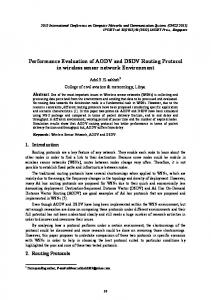
Figure 1: Pursue Mobility Model
Table 1: Algorithm for Pursue Mobility Model
In order to arrive total mobility metric, M, for a scenario, the mobility measure in Equation 2 is averaged over all node pairs, resulting in the following definition M=
1 n X X 1 X 2 Mxy = Mxy | x, y | x,y n(n − 1) x=1 y=x+1
4. If distance P (xi , yi ) < distance T (tx , ty ).
Algorithm
Pursue mobility model and its algorithm is presented in this section. The pursue mobility model attempts to represent MNs tracking a particular target. For example, this model could represent the scenario where police officers attempt to catch a escaped criminal. The Pursue mobility model consists of an update equation for the new position of each mobile node: new position = old position+ acceleration(target old position) + random vector. The current position of a MN, a random vector, and an acceleration function are combined to calculate the next position of the MN. Where acceleration(target old position) is information on the movement of the MN being pursued and random vector is a random offset for each MN. The random vector value is obtained via an entity mobility model. The amount of randomness for each MN is limited in order to maintain effective tracking of the MN being pursued. Figure 1 illustrates the movements of mobility nodes using the pursue mobility model. The white nodes represent the node being pursued and the black nodes represent the pursuing nodes.
ISBN: 978-988-17012-1-3
2. Iterate i = 1,2...,n nodes. 3. Register the location of pursuing node P (xi , yi ).
(3)
where| x, y | is the number of distinct node pairs (x,y) and n is the number of nodes in the scenario. (Note that the second relation in Equation 3 assumes nodes being numbered from 1 to n). The mobility expresses the average relative speed between all nodes in the network. Consequently, the mobility for a group of nodes standing still, or moving in parallel at the same speed, is zero.
4
1. Register the location of target node T (tx , ty ).
5. Set the new position of P (xi , yi ) by updating current pursuing node P (xi , yi ) by acceleration and direction of previous target node position and random offset value. 6. Until P (xi , yi ) catches the target node T (tx , ty ).
The main objective of this algorithm is target tracking, that is collection of nodes P (xi , yi ), trying to chase a single target node T (tx , ty ) as developed and is shown in Table I. Initially, register the location of the target node and individual pursuing node. If the distance between target node and pursuing node is more, then new position of the pursuing node P (xi , yi ) is updated by acceleration and direction of previous target node position and random offset value until it traces the target node.
4.1
Performance Evaluation
This section describes the simulation and experimental results of impact of mobility models on the performance of Ad Hoc On-Demand Distance Vector routing protocol. We have selected packet delivery ratio, latency, throughput as metrics during the simulation in order to evaluate the performance of AODV routing protocol. P acket Delivery Ratio: This is defined as the ratio of the number of packets received by the destinations to those sent by the CBR sources. Latency: This is defined as the delay between the time at which the data packet was originated at the source and the time it reaches the destination. Delays due to
IMECS 2008
Proceedings of the International MultiConference of Engineers and Computer Scientists 2008 Vol II IMECS 2008, 19-21 March, 2008, Hong Kong
route discovery, queuing, propagation and transfer time are included in the delay metric.
Simulation Setup
We carry out the simulation in the customized event driven simulator, OMNET++ [12], which is an object modular network test-bed in C++. The mobility scenarios are obtained through mobility framework which is a part of OMNET++ distribution. The scenario generator produces the different mobility patterns such as Pursue group mobility model and Random Walk, Random Direction, Random Waypoint entity mobility models. In all these patterns 25 hosts with 5 enabled nodes deployed in a simulation area of 700m * 700m rectangular region for 900s simulation time. For our study, we considered a scenario with three random based (i.e., Random Walk, Random Waypoint, Random Direction) entity mobility model, Pursue group mobility model and AODV routing protocol. The scenario is chosen in such a way that, each mobility node speed is varied from 1m/s to 20m/s. From this scenario we compare the performance of AODV routing protocol using entity and group mobility models. The MAC layer protocol IEEE 802.11 is used in simulation with the data rate 11Mbps. The data traffic source to be a Constant Bit Rate (CBR) source. The sending rate is set to three packets per second, the network contains one source and one destination, each message packet size of 512 bytes is defined. The Table II provides all the simulation parameter values.
Packet Delivery Ratio (%)
4.2
RW RWP RDIR PURSUE
0.9 0.8 0.7 0.6 0.5 0.4 0
5
10
5 RW RWP RDIR PURSUE
4
3
2
1
0 0
5
10
15
20
Speed (m/s)
Figure 3: Latency and Speed
RW RWP RDIR PURSUE
8e+06 7e+06 Throughput
700m * 700m 11Mbps 10µsec 900s 5 25 3packets/sec 64packets 512byte 1MB
20
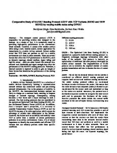
Figure 2: Packet Delivery Ratio and Speed
Table 2: Summary of the communication parameter values for Simulation scenarios Map Size Channel Bandwidth Channel Delay Simulation Time No. of Enabled Nodes Number of Hosts Packet Rate Burst length Message Packet Size Input Buffer Size
15
Speed (m/s)
Latency
T hroughput: The throughput data reflects the effective network capacity. It is defined as the total number of bits successfully delivered at the destination in a given period of time.
1
6e+06 5e+06 4e+06 3e+06 2e+06 0
4.3
5
10 Speed (m/s)
15
20
Results and Analysis
From the simulation results, we compare random based entity models and pursue group model which significantly
ISBN: 978-988-17012-1-3
Figure 4: Throughput and Speed
IMECS 2008
Proceedings of the International MultiConference of Engineers and Computer Scientists 2008 Vol II IMECS 2008, 19-21 March, 2008, Hong Kong
influences the performance metrics such as Packet Delivery Ratio, Latency, and Throughput of AODV reactive routing protocol. The results obtained from the scenario is discussed below. The scenario is based on speeds of nodes varying from 1m/s, 5m/s, 10m/s, 15m/s, 20m/s of mobility models. Figure 2 describes the variation of Packet Delivery Ratio with the speed. As the speed increased from 1m/s to 5m/s Random Waypoint model decreases drastically because of packet loss. By comparing all random based mobility models, the pursue group mobility model shows consistent packet delivery ratio as node speed increased from 1m/s to 20m/s. Figure 3 gives the variation of Latency with speed. Random Waypoint model takes 40% more time to transmit packets as the speed increases upto 10m/s. At a node speed 20m/s, Random Direction model and Pursue mobility model shows better performance than Random Waypoint mobility model. Pursue mobility model experiences 0.1% of consistent time delay as the node speed is increased from 1m/s to 20m/s. This infers pursue mobility model takes less duration to transmit the data among all mobility models. Figure 4 shows the variation of Throughput with speed. The throughput of Random Direction model and Random Waypoint mobility model decreases drastically at node speed 5m/s. It is noticed that, Random Direction model and Pursue group mobility model starts converging as the node speed increases from 10m/s, shows that improvement in Random Direction model in data throughput. From the simulation result, pursue mobility model results in consistent data throughput with variation of speed.
5
Conclusions and Future Work
WSN is gaining importance in the real world because of its applications. In this paper, the simulation results demonstrates the evaluation of performance of AODV routing protocol with random based entity mobility model and pursue group mobility model. The performance metrics are Packet Delivery Ratio, Latency, and Throughput. We intend to show that the choice of mobility models makes the difference with respect to network performance. We have considered a scenario by varying the speed of the individual nodes. The pursue group mobility model performs better than random based entity mobility models. Other mobility patterns such as Freeway, Manhattan, Column group mobility model, City Section models will be used to illustrate realistic situations, in the future works.
ISBN: 978-988-17012-1-3
References [1] Ian F. Akylidiz, Weilian Su, Yogesh Sankarasubramaniam, and E. Cayirci. “Wireless Sensor Network: A Survey on Sensor Networks,” IEEE Communication Magazine, V40, N8, pp. 102-114 8/02. [2] S. Tilak, Nael B. Abu-Ghazaleh, Wendi Heinzelman. “A Taxonomy of Wireless Microsensor Network Models,” Mobile Computing and Communications Review, V6, N2, pp. 28-36, 2002. [3] K. Sohrabi, J. Gao, V. Ailawadhi and G. J. Pottie. “Protocols for Self-Organization of Wireless Sensor Network,” IEEE Personal Communication Magazine, V7, N5, pp.16-27, 10/00. [4] T. He, John Stankovic, Chenyang Lu, Tarek Abdelzaher. “SPEED: A stateless protocol for RealTime Communication in Sensor Networks,” Proceedings of Int Conf on Distributed Computed Systems, Providence, RI, 5/03. [5] M. Ali, T. Suleman, and Z. A. Uzmi. “MMAC: A Mobility-adaptive, Collision-free MAC Protocol for Wireless Sensor Networks,” Proceedings of 24th IEEE IPCCC, 2005. [6] E. Royer and P. Melliar-Smith and L. Moser. “An Analysis of the Optimum Node Density for Ad hoc Mobile Networks,” Proceedings of IEEE Int Conf on Communications (ICC), Helsinki, Finland, 6/01. [7] Guolong Lin, Guevara Noubir, and Rajmohan Rajamaran. “Mobility Models for Ad-hoc Network Simulation,” Proceedings of INFOCOM, 2004. [8] F. Bai, N. Sadagopan, and Ahmed Helmy. “The IMPORTANT Framework for Analyzing the Impact of Mobility on Performance of Routing Protocols for Ad hoc Networks,” IEEE Information Communications Conference, INFOCOM, pp. 825-835, 4/03. [9] J. Broch, D. Maltz, D. Johnson, Y. Hu, and J. Jetcheva. “A Performance Comparison of MultiHop Wireless Ad Hoc Netowrk Routing Protocols,” Proceedings of the Fourth Annual ACM/IEEE Int Conf on Mobile Computing and Networking (MOBICOM), pp. 85-97, 10/98. [10] C. Perkins. “Ad Hoc on Demand Distance Vector (AODV) Routing IETF,” Internet Draft: draft-ietfmanet-aodv-00.txt, 11/97. [11] M. Sanchez. “Mobility Models,” www.disca.upv.es/misan/mobmodel, 2000.
URL:
[12] Andras Varga. Technical University of Budapest, Department of Telecommunications (BME-HIT). “OMNET++ Simulator,” URL: http://www.omnetpp.org/tutorial, 2003.
IMECS 2008