PERFORMANCE OF THE SHEWHART CONTROL CHART FOR MULTIPLE STREAM PROCESSES 1
VADHANA JAYATHAVAJ, 2ADISAK PONGPULLPONSAK 1
College of Oriental Medicine, Rangsit University Thailand, Faculty of Science, King Mongkut's University of Technology Thonburi, Thailand E-mail:
[email protected],
[email protected]
2
Abstract— The multiple stream processes (MSP)of independent identical production units with only single quality control station are generally founded in small business enterprises. The observation units come from each production unit with their probability distributions.The probability density function of the type I error are presented to demonstrate when the observations from individual stream are mixed together. The simulation study in performance of the Shewhart X bar control chart in terms of average run length ( ARL ) and standard deviation of run length ( SDRL ) (when each stream has process mean shifted in times of standard deviation) had been done. The results show that ARL of individual stream control has better than the ARL of the mixed sample monitoring. Index Terms— Average Run Length, Multiplestream processes, X Control Chart.
in the production of consumer products and in services activities i.e., packaged food, plastic, pharmaceutical, bank tellers, supermarket cashiers, etc. The output of one (or a few stream) has shift off target or the output of all streams has shift off target are the two situations of assignable causes in MSP [2]. In 2015, the literature review on statistical control of multiple-stream processes starting from Group Control Chart (GCC) in 1950 to the complicated filling process in 2013 was done by Epprecht [3]. In the GCC the same sample size form each stream are collected and the largest mean and smallest means from all the streams are plotted on the group control chart. If the means are inside the control limits, then all other means will also lie inside the control limit [2]. The adaptive fractional sampling approach was applied to high-speed filling machines of 52 independent streams filling operation [4]. One chart for each stream has the disadvantage, as the number of streams increase more charts are required, however, the nonconformities can be detected from the probable stream directly. In the GCC, detection capability for those streams may decrease [5]. The control charts to monitor multiple stream processes based on F test and a likelihood ratio test have been proposed in 2008 [6]. The guideline and a case study of selecting MSP control charts by considering the major factors, which are correlation among streams, number of streams, limitation to use one chart per stream, difference among streams average, and shift size of streams average to be detected [7]. The chart for enhanced detecting of shifts in one stream proposed in 2011 [8]. The related MSP articles have been proposed for larger number of streams and the machine operates at a rate too great for a sample to be taken from each stream at given point in time. Adding a new machine or 2-3 machines to produce the same product with or without adjust quality control operation is the capacity expansion in small business enterprise (SME). The individual stream quality
I. INTRODUCTION Applying scientific principles to control a variable quality, the Shewhart control chart was first proposed by Walter A. Shewhart since 1920s [1]. For the quality characteristic (say w ) with the mean w and the standard deviation w , then the center line is w , the control limit is w L w , where L is the distance of the control limits from the center line, expressed in standard deviation units. For the normally distributed characteristic with mean and standard deviation , the X control chart with a sample size of n that has as the center line and Z / 2 x as the control limit. The and can be estimated from the samples when process is in control. The performance of the X chart is the average run length ( ARL ), the in control ARL ( ARL0 ) is the number of consecutive samples which their x plots within the control limit until one point plots out of control, that ARL0 1 /
(1)
where is the type I error probability. The six sigma control limit (within 3 ) for normal distribution has = 0.0027, ARL0 is 370 [2]. And the assignable cause occurs the process change to out of control, the out of control ARL ( ARL1 ) is computed from the producers’, that is ARL1 1 / (1 ) (2) where is the type II error probability. A multiple stream process (MSP) is a process with producing the identical product from several individual sources or streams [2]. MSP can be found
Proceedings of 66th The IIER International Conference, Seoul, South Korea, 31st March 2016, ISBN: 978-93-85973-88-8 17
Performance of the Shewhart X Control Chart For Multiple Stream Processes
distribution [2].The normal probability plot of 10,000 average run length plots from N(0,1) with the given -/+ 3 control limit ( = 0.0027) and the sample size of n =5 is shown in Fig. I. The ARL0 of N(0,1) with the given -/+ 3 control limit from 30,000 run lengths simulation for n = 3,4, and 5 are 374.3, 374.3, and 367.6 respectively, ARL0 from simulations are closed to 370 (1/0.0027).
monitoring policy (an individual x chart for each stream or monitoring x i , for i =1,…, m streams) has an advantage in detecting nonconformity from each stream directly, but with additional quality management. If the process monitor the whole process without separating the samples (combine samples from every stream together (monitoring x A )), the sample gathering activity will be easier, but the mixed processes distribution ( x A distribution) will be different from individual stream probability distribution ( x i distribution) and also affect the type I error ( ) which lead to different in individual stream performance with overall process performance. To delineate the performance of X control charts in small number of streams production (only two in this study, m =2) by using an individual control chart for each stream ( x i , i =1,2) and the whole processes control chart that mixed the observations together ( x A ). This study compares ARL and SDRL of the multiple stream processes when the process mean of one stream or both streams are shifted. The next section provides the nature of X chart for individual stream and when the two streams mixed together. The subsequence section gives the steps for the X performance simulation. Next, ARL and SDRL computational results of the given multiple stream processes are compared. Finally, the conclusions and scope for future research complete the paper.
B. Two Individual Distributions and Mixed Distrbution Producing the same target quality (the same control limit) from every stream, if X computes from the observations collected from every stream for m number of streams, the overall stream ARL0 ( ARL 0 ) may differ from the individual ARL0 . In the case that some or all streams may shift from their mean, the
ARL 0 performance will also different from individual stream because the additional overlapped probability distribution (larger 1 rejection region) comes from the shifted stream. The illustration on the individual stream distribution and mixed streams distribution are shown Fig. II and Fig. III below. The individual density function of N(0,1) and N(1.5,1) are shown in Fig. II. The equaled observations mixed streams distribution from N(0,1) and N(1.5,1) , 25,000 random numbers from each stream have, the mixed density is shown in Fig. III (a),the mixed mean = 0.7519 and the mixed standard deviation = 1.2459. The plot of normal density of the mixed distribution is shown in Fig. III (b).
II. SHEWHART X CHART FOR MULTIPLE STREAM PROCESSES
Normal(0,1) 0.4
A. Average Run Length Distribution In general quality control situation, the samples are collected from each independent production unit (PU) with the same quality target. The x i is plotted on its separated control chart for each stream separately, the performance of each stream will correspond to the control limit from the determinedtype I error ( ), ARL0 1 / .
0.35 0.3 0.25 0.2 0.15 0.1 0.05 0 -5
Normal Probability Plot
0.999 0.997 0.99 0.98 0.95 0.90 Probability
-4
-3
-2
-1
0
1
2
3
4
5
n2 =5).
Fig. II The densities of N(0,1) and N(1.5,1) with ( n1 -3
4
x 10
3.5
0.75 0.50
3
0.25 0.10 0.05 0.02 0.01 0.003 0.001
2.5 2 1.5 0
500
1000
1500 Data
2000
2500
3000
1
Fig. I The normal probability plot of 10,000 average run length plots from N(0,1) n=5.
0.5 0 -5
ARL0 is the geometric random variable with parameter and 1 / is the mean of this geometric
-4
-3
-2
-1
0
1
2
3
4
5
(a) The density of mixed N(0,1) and N(1.5,1) from the simulation of 25,000 random numbers each.
Proceedings of 66th The IIER International Conference, Seoul, South Korea, 31st March 2016, ISBN: 978-93-85973-88-8 18
Performance of the Shewhart X Control Chart For Multiple Stream Processes
A. The Sample Size ni = the sample size of the stream i for i 1, 2 . n A n1 n2 = the sample of the mixed stream.
Normal(0.75,1.24) 0.35
0.3
In this case: n1 n2 n , then n A 2 n . B. ARL and SDRL ARLi is the mean of run length of the stream i . ARLA is the mean of run length of the mixed stream. SDRLi and SDRLA are the standard deviation of ARLi and ARLA . C. Algorithm for Each Run Length C.1 Individual Stream For each run length, set RL =0, and repeat the steps below, 1: Generate n random number from N( ,1) 2: Compute x i 3: If x i plots within CLi , then RL RL 1 else break. C.2 Mixed streams For each run length, set RL =0, and repeat the steps below, 1: Generate n random number from N( ,1) from Stream 1. 2: Generate n random number from N( ,1) from Stream 2. 3: Compute x A 4: If x A plots within CLA , then RL RL 1 else break.
0.25
0.2
0.15
0.1
0.05
0 -5
-4
-3
-2
-1
0
1
2
3
4
5
(b) The density of equally mixed N(0,1) and N(1.5,1) or N(0.7518, 1.2459). Fig. III The distribution of mixed N(0,1) and N(1.5,1).
III. THE X CONTROL CHART In the m streams process, the X control chart for the individual stream monitoring ( xi , ni ) using the sample mean x i with the sample size ni , for i 1,.., m and the mixed or overall streams monitoring ( x A , nA ) using the sample mean x A with the sample size nA . Given the mean ( ) the standard deviation ( ) of the underlying process distribution are known, then
V. NUMERICAL SOLUTIONS A. Individual Stream Performance The ARL and SDRL of an Individual stream N(0,1) with 3 control limit for the sample size n = 3,4, and 5 and shift in times of standard deviation ( =0.0,0.5,1.0,1.5,2.0,2.5, and 3) for 30,000 run lengths simulation are shown in Table I. Table I. Performance of an Individual stream N(0,1) with shift 30000 run lengths simulation. IV. TWO STREAM PROCESSES X CHART PERFORMANCE EVALUATION This study evaluates performance of the two independent production units ( m 2 ) with the same rate of output, the underlying process distribution of each stream is the standard normal distribution N(0,1) with 3 control limit, and the process mean of each production unit can be shift in times of standard deviation where = 0.0, 0.5, 1.0, 1.5, 2.0, 2.5, and 3. In this study the term ARL is used in both in control (when the mean of both processes are 0) and out of control average run lengths (when at least one stream has mean shift from 0). The ARL and SDRL from each mean shifts combination is evaluated through simulation. Proceedings of 66th The IIER International Conference, Seoul, South Korea, 31st March 2016, ISBN: 978-93-85973-88-8 19
Performance of the Shewhart X Control Chart For Multiple Stream Processes
individual stream control, if the probability of process B. Mixed Stream Performance The mixed streams in this study n1 = n2 = 5= n , then n A =10. The ARL and SDRL of the two independent stream processes of N(0,1) with 3 control limit for the sample size n1 = n2 = 5= n and both stream process means can be shifted in times of standard deviation ( =0.0,0.5,1.0,1.5,2.0,2.5, and 3) for 30,000 run lengths simulation are shown in Table II.
m
i to be out of control is 1- i , then
(1 ) i
is the
i 1
probability that at least one process out of control. The overall performance will affect by weight from the proportion of sample size of the shift streams. Suggested further research direction for the multiple stream processes with small number of streams which the underlying process distribution might not be identified clearly (in a distribution free control charts ) and the in the short production run causes from flexible manufacturing requirements, the research will worth for those quality control operation in small business enterprises.
TableII. Performance of the Mixed Stream Processes ( n1 = n2 = 5= n , nA = 10)
ACKNOWLEDGEMENT V. Jayathavaj thanks College of Oriental Medicine, Rangsit University for their fully support. REFERENCES [1]
[2] [3]
[4]
CONCLUSION [5]
The average run lengths of an individual stream ( n = 5 ) or ARLi of are 367.6, 32.6, 3.5, 0.6, 0.1, 0.0, and 0.0 for =0.0,0.5,1.0,1.5,2.0 ,2.5, and 3 respectively (Table I.). The average run lengths of the mixed streams ( n1 = n2 = 5, nA 10) or ARLA when only one process mean shifts are 368.3,72.7, 11.9, 2.8, 0.8, 0.2, 0.0 for =0.0,0.5,1.0,1.5,2.0,2.5, and 3.0 respectively
[6]
(Table II.). The individual stream monitoring ( xi , ni for i 1,.., m ) has higher performance than the overall
[8]
[7]
streams monitoring ( x A ). For a multiple stream processes with independent streams using an
W.A. Shewhart, “Economic Control of Quality of Manufactured Product”, Journal of the American Statistical Association, Vol. 27, No. 178 (Jun., 1932), pp. 215-217, 1932. D.C. Montgomery, “Statistical quality control 7th edition,” WILEY, 2013. E.K. Epprecht, “Statistical control of multiple-stream processes: a Literature review, ” Frontiers in Statistical Quality Control 11, pp. 49-64, Springer International Publishing, 2015. J.W. Lanning, D.C. Montgomery, G.C. Runger, “Monitoring a multiple stream filling operation using fractional samples ,” Quality engineering, Vol. 15, No. 2, 2002-3, pp. 183-195, 2002. N.S. Meneces, S.A. Olivera, C.D. Saccone, J. Tessore, “Statistical control of multiple-stream processes: a Shewhart control chart for each stream,” Quality engineering, Vol. 20, No. 2, Apr-June 2008, pp. 185-194, 2008. X. Liu, R.J. Mackay, S.H. Steiner, “Monitoring multiple stream processes,“ Quality engineering, Vol. 20, No. 3, June 2008, pp. 296-308, 2008. P. Jirasettapong, N. Rojanarowan, “A guideline to select control charts for multiple stream processes control,”, Engineering Journal, Vol. 15, No. 3, pp. 1-14, 2011. DOI: 10.4186/ej.2011.15.3.1 E.K. Epprecht, L.F. Marques Barbosab, B.F. Teixeira Simõesc, “SPC of multiple stream processes – a chart for enhanced detection of shifts in one stream,” Produção, Vol. 21, No. 2, pp. 242-253, abr./jun. 2011, 2011.
Proceedings of 66th The IIER International Conference, Seoul, South Korea, 31st March 2016, ISBN: 978-93-85973-88-8 20