Performance Prediction of a Turbo-coded Link in Fading Channels

AALTO UNIVERSITY SCHOOL OF SCIENCE AND TECHNOLOGY Department of Communications and Networking

Muhammad Moiz Anis

Performance Prediction of a Turbo-coded Link in Fading Channels

Master’s Thesis submitted in partial fulfillment of the requirements for the degree of Master of Science in Technology.

Otaniemi, Espoo. March 23rd , 2010

Supervisor:

Professor Olav Tirkkonen

Instructor:

Helka-Liina Määttänen, M.Sc. (Tech.)

AALTO UNIVERSITY SCHOOL OF SCIENCE AND TECHNOLOGY Author:

ABSTRACT OF THE MASTER’S THESIS

Muhammad Moiz Anis

Name of the Thesis: Performance Prediction of a Turbo-coded Link in Fading Channels Date:

March 23rd , 2010

Department:

Department of Communications and Networking

Professorship:

S-72

Supervisor:

Prof. Olav Tirkkonen

Instructor:

Helka-Liina Määttänen, M.Sc. (Tech.)

Number of pages: 78

Channel coding is the method of adding redundancy to the data in order to reduce the frequency of errors or to increase the capacity of a channel. Turbo codes are the most superior class of codes making achievable channel capacity almost at par with the Shannon limits. In Adaptive Modulation and Coding (AMC) the prediction of error performance of a channel is an important step before choosing one of the Modulation Coding Scheme (MCS). Since in Turbo-coded system we donot have analytical relations to relate error performance with the Signal to Noise Ratio (SNR). Therefore, normally simulation results are stored in the form of the look up tables.

In this work we propose an error performance prediction model for a BPSK modulated Turbo-coded link. This model predicts performance addressing the fading phenomena for wireless radio channels. It takes the large variations in the SNR level within a code block into account along with the coding parameters. The SNR dB values profile inside a code block is considered in terms of their mean and variance. The model proposed is UMTS compliant and is continuous for values of the MCS code rate and the mean and variance of SNR dB values. It is an easier way of predicting link level performance as it replaces the discrete look up tables. Unlike the look-up tables it can be used for differentiation based analytical techniques used in system level optimization.

Keywords: Fading, BLER, effective SNR, mean, variance, Turbo-codes.

ii

I would like to dedicate this work to the most perfect human being God ever created (according to my belief ), the Prophet Muhammad (May peace be upon him)

iii

Acknowledgments The driving force behind me, from the ideal evolution till the accomplishment of the realized targets in this work is my thesis supervisor Professor Olav Tirkkonen. His support and confidence was an asset for me. In fact there were numerous occassions where his presence as a devoted mentor helped me greatly in maintaining my focus. His personality has always been a source of inspiration. I put forward my most heartfelt gratitudes to him for being an examplery researcher. As a supervisor he was so kind to accomodate me despite his busy schedule, for any sort of consultation regarding this work. I offer my earnest thanks to him for being a staunch supporter of every aspect of this work. My thesis instructor MSc. Helka-Liina Määttänen also deserves my sincere thanks for being very cooperative, supportive and friendly. I am in particular thankful for the frequent reviews she did of this draft. Inspite of having her work seat in Nokia Research Center (NRC), I feel indebted for her firmness in commitment and devotion to this work. In particular her advice regarding research work writing has proven to be highly valuable. I am grateful to her for support and guidance in every phase of this work. Apart from these two personalities there are two other people who were also kind enough to help technically at various stages of this work. They are Mr. Kalle Ruttik and Mr. Sergio Lembo. Being my seniors, both were helpful in providing their valuable advice and support. Particularly, Sergio deserves a special thanks for providing his assistance in issues regarding the simulations involved in this work. I would like to thank my roommates in the office: Anzil Abdul Rasheed, Iiro Jantunen and Alexander Renaud Pitawal for their pleasant and favourable presence throughout this work. It was always nice to listen about the Nordic and Finnish history from Iiro and chatting with Anzil during leisure time. Anzil was decent enough to give iv

his advice in particular about thesis writing in Latex. I am indebted to Mr. William Martin also for undertaking a thorough and valuable language check up of this draft. I regard my friends Umar, Maliha, Khurram, Zohaib and Farhan also for keeping me cheered up with their invigorating and joyful company. I feel indebted to my parents for providing me with the best education, despite their limited resources, and carving a dignified character out of myself. Here, I cannot skip a whole-hearted thanks to the Finnish Government’s policy of free education for foriegn students. It is laudable on part of the Finnish researchers’ community also who welcomes foriegn researchers and students with open arms and gives them a chance to integrate and excel.

Otaniemi, Espoo. March 23rd , 2010

Muhammad Moiz Anis

v

Contents Abbreviations

ix

List of symbols

xi

List of Figures

xvii

List of Tables

xviii

1 Introduction

1

1.1

Background . . . . . . . . . . . . . . . . . . . . . . . . . . . . . . . .

1

1.2

Contribution . . . . . . . . . . . . . . . . . . . . . . . . . . . . . . .

4

1.3

Structure and Organization . . . . . . . . . . . . . . . . . . . . . . .

5

2 Turbo coding 2.1

8

Introduction . . . . . . . . . . . . . . . . . . . . . . . . . . . . . . . .

8

2.1.1

Birth of Turbo codes . . . . . . . . . . . . . . . . . . . . . . .

8

2.2

Block Codes . . . . . . . . . . . . . . . . . . . . . . . . . . . . . . . .

9

2.3

Convolutional codes . . . . . . . . . . . . . . . . . . . . . . . . . . .

11

2.3.1

Convolutional Encoder . . . . . . . . . . . . . . . . . . . . . .

11

2.3.2

Viterbi Decoding algorithm . . . . . . . . . . . . . . . . . . .

14

Turbo Codes . . . . . . . . . . . . . . . . . . . . . . . . . . . . . . .

15

2.4.1

Turbo Encoder . . . . . . . . . . . . . . . . . . . . . . . . . .

17

2.4.2

Turbo Decoding . . . . . . . . . . . . . . . . . . . . . . . . .

18

2.4.3

Maximum A-Posteriori (MAP) Decoding Algorithm . . . . .

21

2.4.4

MAP Derivatives: Log MAP and Max Log MAP . . . . . . .

23

2.4.5

Soft Output Viterbi Algorithm (SOVA) for decoding . . . . .

25

2.4

2.5

Conclusion

. . . . . . . . . . . . . . . . . . . . . . . . . . . . . . . . vi

25

3 Error Performance of Turbo-coded BPSK Link

26

3.1

Shannon´s Error Free Channel . . . . . . . . . . . . . . . . . . . . .

26

3.2

Error Performance of Memory-less Modulation Signals . . . . . . . .

27

3.2.1

Binary Modulation Systems . . . . . . . . . . . . . . . . . . .

27

3.2.2

BPSK Modulation System in Fading Channel . . . . . . . . .

30

Turbo Coded BPSK . . . . . . . . . . . . . . . . . . . . . . . . . . .

30

3.3.1

AWGN or Non-Fading Channel . . . . . . . . . . . . . . . . .

31

3.3.2

Fading Channel . . . . . . . . . . . . . . . . . . . . . . . . . .

35

3.3

3.4

Conclusion

. . . . . . . . . . . . . . . . . . . . . . . . . . . . . . . .

4 Performance Prediction and Fading

36 38

4.1

Adaptive Modulation and Coding . . . . . . . . . . . . . . . . . . . .

39

4.2

Performance Prediction . . . . . . . . . . . . . . . . . . . . . . . . .

40

4.3

Fading channel . . . . . . . . . . . . . . . . . . . . . . . . . . . . . .

42

4.4

Varying SNR and Fading . . . . . . . . . . . . . . . . . . . . . . . .

42

4.4.1

Effective SNR Mapping . . . . . . . . . . . . . . . . . . . . .

43

4.4.2

Performance prediction Model for Fading Channels . . . . . .

44

4.5

Conclusion

. . . . . . . . . . . . . . . . . . . . . . . . . . . . . . . .

5 Link Simulations

46 47

5.1

Link Layout . . . . . . . . . . . . . . . . . . . . . . . . . . . . . . . .

47

5.2

Two-peak Distribution . . . . . . . . . . . . . . . . . . . . . . . . . .

49

5.2.1

Mean and Variance Expressions . . . . . . . . . . . . . . . . .

50

5.2.2

Channel Coefficients . . . . . . . . . . . . . . . . . . . . . . .

51

5.3

Simulator Structure . . . . . . . . . . . . . . . . . . . . . . . . . . .

51

5.4

Simulation Issues . . . . . . . . . . . . . . . . . . . . . . . . . . . . .

53

5.4.1

1000 snapshots approach and smoothness in performance curves 54

5.4.2

Linear average dB represented SNR on x-axis . . . . . . . . .

55

5.4.3

Curves for UMTS standard Turbo code in fading channels . .

55

5.4.4

Results Analysis . . . . . . . . . . . . . . . . . . . . . . . . .

55

5.5

SNR statistics vs Effective SNR value . . . . . . . . . . . . . . . . .

58

5.6

Conclusion

58

. . . . . . . . . . . . . . . . . . . . . . . . . . . . . . . .

6 Curve Fitting

60

vii

6.1

Heuristic selection of a Sigmoid function . . . . . . . . . . . . . . . .

60

6.2

Modifications in Sigmoid function . . . . . . . . . . . . . . . . . . . .

61

6.2.1

G-factor . . . . . . . . . . . . . . . . . . . . . . . . . . . . . .

62

6.2.2

Flooring Effect . . . . . . . . . . . . . . . . . . . . . . . . . .

63

6.3

Cross Relationship between Code Rate and SNR Variance . . . . . .

65

6.4

Proposed Function . . . . . . . . . . . . . . . . . . . . . . . . . . . .

65

6.5

About Fitting Method . . . . . . . . . . . . . . . . . . . . . . . . . .

66

6.5.1

. . . . . . . . . . . . . . . . . . . . . . . . . .

66

6.6

Optimal Form of the Function . . . . . . . . . . . . . . . . . . . . . .

67

6.7

Conclusion

. . . . . . . . . . . . . . . . . . . . . . . . . . . . . . . .

68

6.8

Prospective Development . . . . . . . . . . . . . . . . . . . . . . . .

72

Fitting Metric

A Parametric Expressions for Four Statistical Numbers

73

Bibliography

76

viii

Abbreviations AMC

Adaptive Modulation and Coding

ARQ

Automatic Repeat Request

AWGN

Additive White Gaussian Noise

BCH

Bose Chaudhuri Hocquenghem

BEC

Backward Error Correction

BER

Bit Error Rate

BLER

Block Error Rate

BPSK

Binary Phase Shift Keying

CODEC

Coder and Decoder

CQI

Channel Quality Indicator

CRC

Cyclic Redundancy Codes

CSI

Channel Side Information

ESM

Effective SNR Mapping

FEC

Forward Error Correction

LLR

Log Likelihood Ratio

LTE

Long Term Evolution

MAP

Maximum A-Posteriori

MCS

Modulation Coding Scheme

ix

MIMO

Multiple Input Multiple Output

OFDMA

Orthogonal Frequency Division Multiple Access

PC

Power Control

PDF

Probability Density Function

RMSE

Root Mean Square Error

RS

Reed Solomon

SOVA

Soft Output Viterbi Algorithm

SSE

Sum of Square Error

UMTS

Universal Mobile Telecommunication System

WiMAX

Worldwide Interoperability for Microwave Access

3G

Third Generation

4G

Fourth Generation

3GPP

3rd Generation Partnership Project

x

List of symbols m

Mean of dB SNR distribution inside Code block

v

Variance of dB SNR distribution inside Code block

m1

Mean of the first constituent distribution of the two peak distribution

v1

Variance of the first constituent distribution of the two peak distribution

m2

Mean of the second constituent distribution of the two peak distribution

v2

Variance of the second constituent distribution of the two peak distribution

p

A fractional number used to control the weightage between the two constituent distributions of the two peak distribution

n

Total number of bits per code block

k

Number of information bits per code block

np

Number of parity bits generated by each constituent encoder

R

Code rate

K

Number of shift registers

xi

CL

Number of bits in encoder memory or constraint length

g

Generator polynomial coefficients vector

g(z)

Generator polynomial

z1

Representing first memory stage or shift register in generator polynomial

z2

Representing second memory stage or shift register in generator polynomial

bi

Input bit

bp

Parity bit

s1

State of first shift register

s2

State of second shift register

J

Stage of time or clock

xk

Set of input information bits for a turbo encoder

0

xk

Set of interleaved version of the input information bits for a turbo encoder

zk

Set of parity bits generated by first RSC encoder

0

zk

Set of parity bits generated by second RSC encoder

uk

Representing an encoded symbol which may be +1 or -1 for a 1 or 0 information or parity bit

L(uk ) y

0

Sk−1

LLR corresponding to each uk Received symbol sequence Previous state of the registers

xii

Sk

Current state of the registers

s

The final state of a considered transition

0

s

The initial state of a considered transition 0

αk−1 (s )

0

The probability of being in state s at time k−1

βk (s)

The probability of being in state s at time k

0

0

ϕk (s , s)

The probability of transition from s to s

γ

Signal to Noise Ratio, SNR

xi

Set of probability numbers to be applied with Max-Log-MAP approximation

fc

Correction factor introduced in Max-LogMAP approximation for Log-MAP

ν

Corrected approximation function by LogMAP

Eb , b

Transmitted (or coded) bit energy

Ebi

Information bit energy

N0

Twice of gaussian noise spectral density

r

Received signal

s0

Signal level associated with a ’0’

s1

Signal level associated with a ’1’

p(r/s0 )

Probability of signal reception given signal transmitted is s0

p(r/s1 )

Probability of signal reception given signal transmitted is s1

d12

Intersymbol distance

Pb

Error probability xiii

rl (t)

Received signal in one signaling interval

sl (t)

Transmitted signal in one signaling interval

η(t)

Received signal in one signaling interval

µ

Amplitude of fading coefficients, considering them as complex numbers

φ

Angle of fading coefficients, considering them as complex numbers

γb

SNR per bit

p(γb )

Probability density function of SNR per bit

P2 (γb )

Bit error for BPSK modulated signals when µ is fixed

Pe

Bit error for BPSK modulated signals when µ is variable

γmean

Mean SNR value

L

Bad estimate of reliability factor

Lc

Correct reliability factor

X

Linear factor i.e. ratio of L to Lc

L(yk |xk )

Conditional log likelihood ratio or Soft output through the channel

a and ak

Fading channel amplitude response coefficient vector

M

Magnitude of signal

BW

Signal bandwidth

yk

Channel ouput vector following matched filter approximation

xiv

σ2

Noise variance

B

Block length

γef f

Effective value of SNR, when channel doesnot have a uniform state inside code block

fSN R (γ)

Probability Density Function (PDF) for continuous channel symbol SNR values

pi

Probability mass function for discrete SNR values

I(γ)

Information measure

N

Number of times loop running for the Monte carlo simulation

S

Skewness of dB SNR distribution inside code block

K

Kurtosis of dB SNR distribution inside code block

c1 -c4 , k1 -k21 0

0

a , a1 , a2 , b , b1 , b2 and G

Parameters used in curve fitting Constant numbers used for illustrative explanation of different curve fitting mechanisms

xv

List of Figures 2.1

Block code composition . . . . . . . . . . . . . . . . . . . . . . . . .

11

2.2

a 0.5 rate Convolutional Encoder with state transition diagram, [14]

13

2.3

Trellis diagram for the Encoder shown in Figure 2.2 . . . . . . . . .

14

2.4

Trellis Viterbi decoding for the encoder shown in Figure 2.2 . . . . .

16

2.5

Turbo encoder comprising of 2 identical RSC encoders [3] . . . . . .

17

2.6

Effect of the number of iterations on BER curve [14] . . . . . . . . .

18

2.7

A typical turbo decoder . . . . . . . . . . . . . . . . . . . . . . . . .

19

2.8

Possible transitions for K=3 RSC encoder [14] . . . . . . . . . . . . .

22

2.9

Possible transitions for K=3 RSC encoder [14] . . . . . . . . . . . . .

23

3.1

PDFs of two binary symbols [25] . . . . . . . . . . . . . . . . . . . .

28

3.2

Error probability comparison for binary signals . . . . . . . . . . . .

29

3.3

Error probability comparison between AWGN and Rayleigh fading channel . . . . . . . . . . . . . . . . . . . . . . . . . . . . . . . . . .

31

3.4

BER performance for different decoding algorithms [14] . . . . . . .

32

3.5

Performance at different code rates realized by different numbers of punctured parity bits, [14] . . . . . . . . . . . . . . . . . . . . . . .

33

3.6

Effect of framelength on BER performance [14] . . . . . . . . . . . .

33

3.7

Effect of channel reliability factor estimation [14] . . . . . . . . . . .

34

3.8

Performance at different code rates realized by different numbers of

3.9

punctured parity bits [14] . . . . . . . . . . . . . . . . . . . . . . . .

36

Performance at different degrees of selectivity realized [12] . . . . . .

37

xvi

4.1

Example AMC scheme for a WiMAX base station . . . . . . . . . .

40

4.2

Example MCS set . . . . . . . . . . . . . . . . . . . . . . . . . . . .

41

4.3

Non-uniform SNR within a code block . . . . . . . . . . . . . . . . .

43

4.4

A comparison among different information measures [27] . . . . . . .

44

4.5

Error performance comparison for two different information measures [27] . . . . . . . . . . . . . . . . . . . . . . . . . . . . . . . . .

45

5.1

Block diagram of the overall Link . . . . . . . . . . . . . . . . . . . .

48

5.2

PDF of a two-peak distribution: p=0.5,m1=-10,m2=5,v1=1,v2=3 .

49

5.3

Block diagram of the simulator . . . . . . . . . . . . . . . . . . . . .

52

5.4

Unreliable curves obtained in first attempt . . . . . . . . . . . . . . .

53

5.5

Smoother curves with scaling problem . . . . . . . . . . . . . . . . .

54

5.6

Plots with linear mean SNR in dB on x-axis . . . . . . . . . . . . . .

56

5.7

UMTS standard compliant curves for various code rates . . . . . . .

57

6.1

Oscillating polynomial fit over some data points . . . . . . . . . . . .

61

6.2

An example Sigmoid curve . . . . . . . . . . . . . . . . . . . . . . . .

61

6.3

A closer Sigmoid curve . . . . . . . . . . . . . . . . . . . . . . . . . .

62

6.4

Sigmoid curves of different slopes . . . . . . . . . . . . . . . . . . . .

62

6.5

Sigmoid curves for changing G in a semilog plot . . . . . . . . . . . .

63

6.6

Sigmoid curves for a known slope and position . . . . . . . . . . . .

64

6.7

Sigmoid curves with different levels of flooring effect . . . . . . . . .

64

6.8

Constant BLER surfaces . . . . . . . . . . . . . . . . . . . . . . . . .

65

6.9

Case 6: Fitting the simulated curves with 21 parameters . . . . . . .

71

xvii

List of Tables 6.1

Explanation of each Case . . . . . . . . . . . . . . . . . . . . . . . .

6.2

Parametric values and correpsonding Fitting metric for cases without G-factor . . . . . . . . . . . . . . . . . . . . . . . . . . . . . . . . . .

6.3

68

69

Parametric values and correpsonding Fitting metric for cases with G-factor . . . . . . . . . . . . . . . . . . . . . . . . . . . . . . . . . .

xviii

70

Chapter 1

Introduction 1.1

Background

In telecommunication applications wireless systems are preferred over wired ones due to easy installation and maintenance, flexibility in reconfiguration, low cost components and mobility. In practice, however, a wireless channel is a less reliable media, in particular because of the fading in the radio channels. A signal in a wireless channel becomes attenuated. Fading can be defined as the variation in that attenuation which may vary with time, geographical location or radio frequency. The variations in the signal strength are classified as large and small scale variations in [28]. Large scale variations, due to average path loss because of the distance trav-

elled and shadowing by large objects such as buildings and hills. This is typically frequency independent. It occurs when mobile moves through a distance of the order of the cell size. Small scale variations, due to the constructive and destructive interference

of the multiple versions of the same signal travelling through different paths between the transmitter and receiver. This type of variation is frequency dependent. The fading channels are normally classified as slow fading and fast fading channels. A channel is said to be fast fading if the coherence time of the channel is much shorter than the delay requirements of the application, and is a slow fading channel if the coherence time is longer. Coherence time can be defined as the minimum time required to make the amplitude changes of signal uncorrelated with its previous 1

CHAPTER 1. INTRODUCTION

2

value [28]. Channel coding is the method of adding redundancy patterns to the signal for lowering the error rate. If the data has too many errors for the desired use, then coding is used to attain a less frequent error rate or to attain a greater data rate. Wireless systems performance have gained enough improvement with channel coding. In particular, with turbo codes achievable throughput is very close to the Shannon limits which was not possible before [15]. The now classic turbo-coding scheme is based on a composite Coder and Decoder, (CODEC) constituted by two parallel concatenated codecs. Since their invention, turbo codes have evolved at an unprecedented pace and have reached a state of maturity in a relatively short time scale. As a result, turbo coding has also been standardized in systems, such as, for example, the third-generation (3G) mobile radio systems. To improve system performance, peak data rate and coverage reliability for a particular link, the transmitted signal is modified to compensate for signal quality variations, a process which is called Link Adaptation. It means changing transmission parameters over a link, such as modulation, coding rate, power, etc., in response to changing channel conditions. It is a powerful means of achieving higher efficiency or throughput in wireless networks. Adaptive Modulation/Coding, (AMC), Adaptive Power Allocation and Water Filling are some of the example of Link Adaptation techniques. According to the literature review in [2], among these techniques AMC is considered attractive because of its simplicity and high performance. The adaptation of the transmission parameters is performed according to the predicted future performance. To render such a performance prediction, there is the need for a realistic model which may give a good prediction of the error rate for a known value of Signal to Noise Ratio, (SNR). Unfortunately, in coded systems analytical relationships, which may define all the resulting performance curves for different combinations of the code parameters like code rate and block length, for instance, are not derivable. Therefore, to study such systems exhaustive computer simulations are required. A comprehensive simulation is essential, but inclusion of modelling of precise phenomena for each of the link


3

been simulated poses huge computational demands. Therefore, there are link and system level type simulations. Link level simulations undertake a detailed modelling of all the steps involved from the generation till the reception and comprehension of digitized information at the receiver passing through the wireless medium. Example phenomena include signal generation, signal encoding, signal modulation, channel modelling, detection and demodulation of the signal as well as signal decoding. The essentiality of segregating simulations is more for the case of turbo-coded systems where in particular the turbo decoding operation is the most resource consuming part of the simulators. The results obtained are often stored in the form of a look-up table or a mathematical function, which are then used in system simulations. System level simulations depict the overall view of a wireless system. In this kind of simulation, all the phenomena at the level of a single link are approximated on the basis of the results coming from link level simulations. Authenticity of system level simulations is dependent on the precision of results at link level. Also the task of optimizing system parameters can be inefficient and difficult if the margin of implementing optimization algorithms over link level results is narrow. For instance, derivative-based optimization techniques can only be used if we have a continuous function, for reproducing link level simulation results. In system level simulations all the link level details are normally hidden behind the relationship defining a system level parameter called Block Error Rate, BLER, defined in terms of Signal to Noise Ratio, which is a link parameter. The first and easier choice for efficient utilization of simulation results would be to maintain lookup tables. But using these will restrict system level simulations for discrete or even a limited set of code rates. A better idea is of forming a mathematical model for performance evaluation. This method of modelling the coded systems’ performance can be found in [19] and [20]. In the mentioned work the channel is considered to be as Additive White Gaussian Noise, (AWGN) channel. In an AWGN channel, where it has a constant additive white noise and amplitude response is 1, SNR mapping is not challenging and the channel within a block does not vary. Therefore, in the mentioned work the performance of coded systems is considered against coding parameters. For instance, the considered coding parameters are code rate, block length and puncturing pattern


4

in [20]. The case with fading is not that simple. In fading channels a block length may experience mutiple channel states. In other words, there may be multiple values of SNR for groups of bits or even bit specific values of SNR inside a code block. The presence of fading mainly deteriorates the performance, but along with this deterioration, SNR to error performance mapping is also vague. In [27] the idea of having an effective SNR is considered. In this work an averaging term called the information measure is introduced which is then defined in five different forms. Finally, it proves a mutual information averaging measure to provide the best results for turbo codes.

1.2

Contribution

The idea is to establish a relationship of the turbo coded system performance with the statistics of the SNR distribution i.e. mean and variance. Here instead of going for a complicated evaluation of the effective SNR, the SNR distribution within a block has been represented by two statistical numbers. In order to trace a relationship of the link performance with the mean and variance of the SNR dB values inside a code block and code rate, a ready made turbo coded link simulator for AWGN channel with Binary Phase Shift Keying (BPSK) as the modulation scheme, was modified for fading channels. In the pursuit of the targetsoutlined above, a straight route would have been to realize various conventional fading realizations and then calculate and record each realizations higher order statistics for simulations. But this strategy would have led to a very exhaustive exercise. Instead, an SNR distribution has been assumed, which is a weighted sum of two normal gaussian distributions. Hence, considering the mean and variance of each of the two distributions with the weightage parameter, there are five parameters (i.e. the mean and variance of the first normal distribution, m1 , v1 , the mean and variance of the second normal distribution, m2 , v2 and the scaling factor p) which are needed to define this distribution. In our investigation we are concerned about the mean and variance of the SNR distribution generated using these five parameters. Therefore, formulae for mean and variance of the distribution were derived in terms of these parameters and two equations were then solved to find each of the five parameters in terms of the mean


5

and variance of the distribution. This enables a SNR number series to be generated for a known set of the mean and variance of the SNR distribution. These SNR numbers are generated in the dB domain. As a final task of this work, we fit curves to the obtained simulation results in order to acheive a mathematical relationship relating SN R to BLER along with taking into account the code rate and variance of the SNR values profile inside the code block. We take a nonlinear Sigmoidal curve with some suitable modifications and fit it over the simulation results in a least square sense, for a modified fitting metric. The modifictaion in the fitting metric is made to suit the semilog plots which are used to plot the SNR vs BLER relationship.

1.3

Structure and Organization

The structure of this thesis is arranged in a fashion to develop a gradual understanding of the topic by first starting with the pedagogical background and research work and then elevating it to a decent demonstration of the model, developed through the course of this work. Therefore, Chapter 2 is devoted to the introduction of turbo codes. In this chapter we explain the historical causes of the birth of turbo codes. In order to appreciate the superiority of turbo codes, it is important to have a good idea of the codes in use in the era prior to turbo codes. Therefore, suitable attention is given to both block codes and convolutional codes as well. In this chapter two of the most well known decoding algorithms: Viterbi and Maximum A Posteriori, (MAP) have also been explained. In Chapter 3, the performance of turbo codes in both fading and non fading channels is the topic. First, performance of uncoded modulation signals is explained. The inclusion of the discussion about uncoded systems has just been made to make the reader appreciate the ample contrast between the performance of a coded and an uncoded systems and to realize the fact that the behaviours of coded systems are studied via simulation plots because of the lack of analytical relations which would have explained performance. The presence of fading causing depreciation in the performance of a radio link is another important issue discussed in this chapter. In Chapter 4, the concept of performance prediction and its importance in the application of link adaptation techniques has been discussed. Apart from the concept of performance prediction, the problem of having multiple SNR values inside


6

a code block has been discussed. Here the established technique of effective SNR Mapping has also been explained along with the presentation of the main idea of this work. A comparative analysis of the two techniques is also undertaken in this chapter. In Chapter 5, the channel model used to characterize fading in terms of the SNR dB mean and SNR dB variance in a turbo coded link simulator has been conceptualized, followed by a prior discussion about the overall link layout and fading affecting the SNR level inside a code block. The concept of the channel model is supported with mathematical relations for terms like Log Likelihood Ratios and channel coefficients. The chapter also contains the practical issues and other findings evolved during the simulations. In Figure 5.7 the final results are demonstrated comprising of several performance curves on a semilog plot between Block Error Rate (BLER) and mean SNR dB, where each curve is associated with a particular code rate and SNR dB variance. Chapter 6, deals with the curve fitting of a heuristically selected mathematical function over the obtained simulation curves. First, the reason for selecting the mentioned function is discussed, then the initial modification introduced to the Sigmoid is explained. The G-factor has been described as the way of changing the slope and position of a Sigmoid. Also the neccessity of having an additional exponential in the denominator has been emphasized to ensure that the Sigmoid also caters for the flooring effect present in the simulation results. In the final step a thorough optimization of all 12 possible combinations have been performed to obtain the best fit. Conclusively, the model obtained as a result of the curve fitting over the simulation results is mouldable by changing the number of the parameters used. Any of the first six cases out of the total twelve, can be used as working model. The choice of the case shall be a trade off between the required accuracy and the maximum affordable numbers of parameters. The reason of not using last six cases is because of the presence of an additional parameter i.e. G-factor which deteriorates fitting instead of improving it. As a prospective work it is possible to undertake an investigation or modelling with higher statistical numbers of the SNR numbers inside a code block. It is essential, if a fair comparison can be done with a common channel for the developed model with


7

effective SNR based predictor. Such comparison may also help in determining the exact number of statistical numbers for SNR values representation (inside a code block) required to define the performance in selective or fading channels.

Chapter 2

Turbo coding 2.1

Introduction

Information bits transmitted through a communication channel are corrupted by channel variations and noise. If there are too many errors the intended message is misunderstood or not undertood at all. There can be two ways to take counter measures. Either the error is recognized only and the erroneous part is lost or errors are corrected through proper Error Correction techniques. There are two strategies followed for error correction, i.e. Forward Error Correction (FEC) and Backward Error Correction (BEC). Forward error correction can be defined as the error correction method in which each dataword is supposed to have some bits dedicated for detecting and correcting errors in the original message. Parallel to that there is another error correction method called the backward error correction method. In this method in the event of any error, the receiver makes a retransmission request to the transmitter.This error control strategy is also called Automatic Repeat Request (ARQ). [6]

2.1.1

Birth of Turbo codes

In 1948 Shannon laid the foundations of error correction coding. He stated the possibility of a nearly error free transmission over realistic channels by adding some auxiliary information. Historically, the birth of turbo codes is followed by the invention of block codes and convolutional codes, both of which shall be explained in detail in Sections 2.2 and 2.3 respectively. The block codes and convolutional codes have passed through different stages of development in the same period of time. For instance, in 1950 Hamming code was the first single error correcting block code devised [13]. During 1955 Elias discovered Convolutional codes [14]. 8

CHAPTER 2. TURBO CODING

9

In 1967 a maximum likelihood estimation algorithm was introduced by Viterbi for decoding convolutional codes. The algorithm was later interpreted by Forney. In 1970 the first practical application of the Viterbi algorithm with convolutional codes was proposed by Heller and Jacobs. The Maximum A-Posteriori (MAP) decoding algorithm was proposed in 1974. This algorithm offers relatively lesser BER, the performance margin between Viterbi algorithm decoding and MAP decoding being very narrow. MAP has been found to be far more complex for implementation, therefore MAP algorithm had been very rarely implemented till the evolution of turbo codes [14]. Around 1960, the first multiple error correcting block code, Bose Chaudhuri Hocquenghem (BCH) was proposed [5], and then later in the same year eponymous Reed Solomon (RS) codes were introduced. The RS codes are a non-binary subset of BCH codes. In 1968 Berlekamp appeared as the one proposing a range of decoding algorithms for the RS and BCH codes [26]. Also from the same era, evidence of soft decision decoding algorithms cannot be neglected. This was mainly proposed by Sweeney and Honary. The RS codes had also been standardized for various applications including CD players and Digital Video Broadcasting. The standardization of FEC for radio mobile systems dates back to the 1980s. During 1993 with the arrival of turbo codes, the operation of communication systems close to the Shannon limits became possible. Turbo codes were also adopted as the standard for the ratified Third Generation (3G) mobile radio systems. Also adopted were the same binary turbo codes in the 3rd Generation Partnership Project (3GPP) Long Term Evolution (LTE) and duo-binary turbo codes in Worldwide Interoperability for Microwave Access (WiMAX) as mentioned in [18], [8] and [30]. And for Fourth Generation (4G) standardization, the presence of turbo codes is certain and is expected to undergo further evolutions.

2.2

Block Codes

Block codes are refered to as (n,k) codes, as it generates n-bits blocks for any k-bits of information. Block codes are defined as one of the error correction codes having a fixed length of encoded block generated by the encoder against a fixed length of


10

input data word. The ratio of the number of information bits k, to the total number of bits n is defined as code rate R is R=

k k . = n k + np

(2.1)

The total number of bits of an encoded block is the sum of the information bits k and the parity bits np , where parity bits are the additional or redundant bits decided according to the coding algorithm. For uncoded case n = k and so there are no parity bits, i.e. np = 0. In a code, a sequence of symbols assembled in accordance with the specfic rules of the code and assigned a unique meaning is called a code word. Linearity for a code can be proven if the sum of the two code words results in a third valid code word of the same coding scheme. Most of the block codes are defined to be linear, the most well-known example of linear block codes being Cyclic codes. This is because the hardware limitaions often make difficult the attainment of long code words. In this regard the cyclic codes are very important in providing a very practical way of attaining long code lengths. Mathematically, a linear code is called cyclic only if a cyclic shift on the code word results in another code word. A well known class of Cyclic codes is Cyclic Redundancy Codes (CRC). CRC helps in detecting all single bit errors, any odd number of errors and a burst of errors if the burst length does not exceed the number of check bits. The two most common examples of block codes are Reed Solomon (RS) and BoseChaudhury-Hockquenghem (BCH) block codes. Both of them are mathematically based on finite field structures. The finite fields have a limited number of elements. The field is supposed to be closed under the operations been defined for it, i.e. the result of any operation on any two elements of the field is also supposed to be an element of the field. Reed Solomon (RS) is a multiple error correcting code. It can be defined as a non-binary sub class of the BCH code. RS code is a cyclic code i.e. any cycle shifted version of a code word is also a code word. Similarly, a linear combination of some code words also forms another code word. A code having code words with parity bits which are easily distinguishable is called Systematic code. For purposes of illustration, we take an example of a systematic


11

Figure 2.1: Block code composition code word. Figure 2.1 shows the composition of a typical block code’s code word. Improvement in the number of correctable errors requires more parity bits to be added, which is not expandable to a very high number due to computational power constraints.

2.3

Convolutional codes

The concept of convolutional coding is more than half a century old. Since the time of inception it has been being considered as one of the few most efficient Forward error correction codes. The name convolutional code result from their resemblance in operation to a filtering or convolution operation. Unlike block codes, however, they can be applied for coding streams of data and the code rate is the same as defined in Equation 2.1.

2.3.1

Convolutional Encoder

Unlike, the block codes where blocks of data are mapped into (longer) blocks of data, in convolutional codes the encoder maps (in principle continuous and infinite) streams of data into more streams of data. This mapping is realized by sending the data streams over linear filters [22]. If the input data stream is unaltered with in the output streams, then the convolutional encoder is said to be systematic. The term recursive or non-recursive associated with the convolutional encoders comes from their resemblance to a typical filter layout. The most important convolutional encoders in the context of iterative algorithm is the binary systematic recursive convolutional encoder [22], since they are the constituent components of the standard turbo codes. Although [14] discusses block code based turbo codes, at low code rate, however, turbo codes with block codes based constituent encoders have high decoding complexity. Particularly, for code rates less than 2/3, turbo codes having convolutional code based constituent encoders are preferred [11].


12

A convolutional encoder is defined by (n, k, K), where K is the number of shift registers, the number of bits in the encoder memory or constraint length, CL is determined by the number of shift register stages affecting the generation of n encoded output bits. L is given as L = K + 1,

(2.2)

To generate n bits we need n polynomial generators. The generator polynomials are constituted by a bit pattern determining the presence, or absence, of a link from each buffering stage. There are three memory or buffering stages in the encoder shown in Figure 2.2, i.e. the buffered input and the two outputs of the two shift registers. As a new bit enters the input, all the three bits in series are right shifted. As an example the generator polynomial for the encoder in Figure 2.2 can be given as g = [111], this is because the only modulo-2 addition block takes input from all three memory stages. The polynomial can be given as, g(z) = 1 + 1z 1 + 1z 2 .

(2.3)

We take the example of a half rate convolutional encoder with a number of information bits, k = 1, R = 1/2 with a memory of three binary stages which makes the number of shift registers to be two, i.e. K = 2 and the convolutional code can be represented as (2, 1, 2). In Figure 2.2(a) this encoder is shown for the first ten clock cycles. The boxes marked s1 and s2 are the shift registers and the addition is a modulo-2 sum operator. Once a bit stages a register, the output then depends on a predetermined manner of the structure of the encoder and the output bit sequece is thus not arbitrary. The number of valid output bit patterns is limited which helps in the decoding process [14]. In Figure 2.2(b) the state transition diagram is presented which demonstrates the possible transitions for each state as function of the incoming information bit, i.e. bi . In Figure 2.2(a) the corresponding parity bit, bp generated against can also be observed for the first ten clock pulses. The considered input bit stream is also mentioned. In Figure 2.2(b) the broken lines represent bi = 1 and for solid line bi = 0. From the inherent constraint, i.e. two shift registers, there are only two possible states where a transition can be made to. Another simpler way to represent the encoder is a trellis diagram. Figure 2.3 shows the trellis for the encoder in Figure 2.2. In Figure 2.3 the bit stream shown in Figure 2.2(a) is considered, the transition


13

(a) 0.5 rate turbo encoder

(b) State Transition Diagram

Figure 2.2: a 0.5 rate Convolutional Encoder with state transition diagram, [14] against bi = 1 is represented with a broken line and vice versa. Moreover, the transitions represented against each Jth stage of time or clock, in the diagram, strictly follows the transition constraints depicted in Figure 2.2(b).


14

Figure 2.3: Trellis diagram for the Encoder shown in Figure 2.2

2.3.2

Viterbi Decoding algorithm

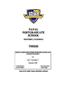
The Viterbi decoding algorithm was proposed in 1967 and it basically performs maximum likelihood decoding, although the computational load is reduced because of the special structure of the code trellis. In order to understand the Viterbi decoding method we need to consider the code trellis shown in Figure 2.4. For simplification, we consider all the zeros bit stream to be transmitted and the received bits have been detected and sent to the decoder. Hamming distance between the two binary numbers is measured in terms of the count of different corresponding bits. In the context of Viterbi decoding this hamming distance is the branch metric. In the Figure 2.4 the two bit number associated to each branch is the encoded ouput number i.e. bi , bp . As in the diagram all possible paths can be found now when the received number enters the decoder in the form of a two bit symbol. It evaluates the cumulative branch metric at every dot if lying on a path. For example, in the Figure 2.4 it received 01 which has a hamming distance of 1 with both possible output numbers 00 and 11 corresponding to the two possible transition states according to Figure 2.2(b), i.e. 00 for bi = 0 and 10 for bi = 1. Note that we assumed the initial state of both of the shift registers to be 00. At this stage, the decoder is unable to express any preference as both paths have the same hamming distance.


15

Proceeding to the second two bit symbol we assume to receive 00 and for this number we have now four candidate branch metrics and they are found to 0,2,1 and 1. The correponding cumulative branch metrics on the four paths at J = 3 are 1,3,2 and 2. At this stage the upper most path can be singled out as the most likely path because of the least distance of the encoded bits to the received bits. This is due to the fact that there exist some finite probability for the other three paths. The third symbol is assumed to be 10 and, accordingly, the cumulative branch metrics are evaluated at this stage. It can be noticed their exist many merging paths giving multiple cumulative branching metric values to the same nodes. In this situation the less likely path or more distant path is dropped, for example at the top node when J = 4 we see a merger of 00, 00, and 00 with the 11, 01 and 01 path. Here the former is kept because of the lesser branch metric and such a path is called a survivor path. Similarly, if two paths merge at a node and give the same metric, then a random selection can be made. In the considered example although it does not affect if any of the path in the bottom at J = 4 in Figure 2.4 is taken. Because the top most path, indicated with a darker line, is already with least cumulative metric value and is supposedly the winning path. In some cases, however, it might lead to errors to have random selections. The decision taken on the basis of the complete information sequence is best, although an early decision help reducing latency. Practically it has been found that the bit error rate is virtually unaffected by curtailing the decision interval to about five times the encoder ’s memory [14] which is three in the discussed example. The associated branch metric for the winning path is also the number of the transmission error. The winning path is the one shown with a darker line in Figure 2.4.

2.4

Turbo Codes

The term Turbo was selected by the inventors in order to emphasize the operation of the codes as reminiscent of the turbo charging of an automobile via engine-heated or exhausted air been fed back to the air intake resulting an increased efficiency. There is a trade off between complexity and performance. By increasing the codelength, the ability of the code to detect and correct error improves but at the same time decoding complexity increases. Also the hardware design faces fierce challenges and constraints due to the limited processing power, specifically for a general purpose processor. Fortunately, turbo codes maintain a very reasonable decoding complexity


Figure 2.4: Trellis Viterbi decoding for the encoder shown in Figure 2.2

16


17

Figure 2.5: Turbo encoder comprising of 2 identical RSC encoders [3] for a very long code length, which has made possible the code performance being almost on par with the Shannon limits, which were hypothetical just before turbo codes were introduced in 1993.

2.4.1

Turbo Encoder

A standard turbo encoder can be thought of comprising a minimum of two convolutional encoders, the most popular choice is Recursive Systematic Convolutional, RSC, encoders. The two RSCs have an inter-leaver between them which makes them statistically independent of each other. Each RSC generates encoded words comprising of some parity bits along with the information bits. These parity bits can then variably be punctured to realize various code rates. As an example, if the two RSCs were half rate, then puncturing half of the parity bits of each RSC makes the overall coderate to be half. Similarly, if both parity bit sets were taken unpunctured then the overall coderate would be one-third. In Figure 2.5 there are two identical RSC encoders, each of them generating a set of parity bits, xk is the set of input information bits with zk which is a set of parity 0

bits generated for xk by the first constituent RSC encoder. Similarly, xk shown in 0

dotted lines is the interleaved version of the input information bits and zk is the set of parity bits generated by the second RSC encoder.


18

Figure 2.6: Effect of the number of iterations on BER curve [14]

2.4.2

Turbo Decoding

One of the most favourable points in the development of turbo codes was the inception of the iterative decoding algorithm. In this algorithm, the decoders iteratively operate on the received data. The greater the number of iterations, the more accurate are the results. Here the a-priori symbol probabilities from the encoder are made available to the first decoder then the rest of the others receive the same probability and send it back to the first, also in a cycle, until some known and predecided number of iterations are completed and finally decide the transmitted code word. The number of iterations increment improves system performance for a very small SNR but there is a limit to that gain. It has been observed that normally after 18 iterations further increase does not reflect significantly on the BER curve. Figure 2.6 depicts BER curves for a different number of iterations. A typical decoder, as shown in Figure 2.7, comprises of two component decoders each decoder taking three inputs. The first input is the systematically encoded channel output bits, the second is the parity bits transmitted from the associated component encoder and the third is the information from the other component decoder about the likely values of the bits concerned. These likely values are also known as the a-priori information from the fellow decoder. This a-priori input comes through an inter-leaver if it is supposed to go to


19

Figure 2.7: A typical turbo decoder a decoder which receives interleaved Systematic input. Similarly, a de-interleaved version of the a-priori information is to be fed to the decoder which takes uninterleaved systematic input. Each decoder is supposed to provide soft outputs along with the decoded bits. During the first decoding attempt, the encoded input is decoded as a soft output and then this soft output is fed to the second decoder which uses this soft output along with the encoded input to give a soft output to be fed to the first decoder which, this time, decodes the encoded input along with soft output from the second cycle. This way it completes the first iteration. There are two popular turbo decoding algorithms, the Maximum A-Posteriori (MAP) and the Soft Output Viterbi Algorithm (SOVA). Log Likelihood Ratios, (LLR) and Reliability Factor The Log Likelihood Ratio of a data bit can be denoted as L(uk ) where uk may assume either +1 or -1. It is merely defined as the ratio of the probabilities of the bit taking its two possible values elaborated mathematically as,

L(uk ) = ln

P (uk = +1) . P (uk = −1)

(2.4)

Prior to decoding, the LLRs have to pass through some channel, where it is essential to understand the importance of the reliabilty factor. For a BPSK modulation


20

case over some channel with the magnitude response coefficient(s) a, in [14] on page 113, the LLR is given as, L(yk /uk ) =

Eb 4ayk , 2σ 2

(2.5)

where L(yk /uk ) is the conditional log likelihood ratio and is also referred as the soft output of the channel. It can be thought of as a product of the matched filter approximated output of the channel denoted by yk , multiplied by the reliability factor denoted by Lc . The reliability factor for the channel is given as, Lc = 4a

Eb . 2σ 2

(2.6)

A matched filter approximated channel output can be expressed as in Equation 2.7. If uk is the encoded signal, ηk is the Gaussian Noise, a is the channel’s magnitude response coefficient, which is equal to ’1’ for as Additive White Gaussian Noise (AWGN) channel, yk = auk + ηk [21].

(2.7)

In [21]on page 239 for a matched filter approximation, a detailed derivation relates Eb N0

and SN R as, SN R =

The

Eb N0

2Eb . N0

(2.8)

used in the simulations for plotting curves is the one taking the informa-

tion bit energy into account. The one considered in Equation 2.6, is related to the coded bit energy. Mathematically, the coded bit energy, Eb is the product of the the information bit energy, Ebi and code rate R, Eb = Ebi R.

(2.9)

Multiplying both sides of Equation 2.9 by twice of the noise spectral density, i.e. N0 , Eb Eb R = i . N0 N0 From Equations 2.8and 2.10, the SNR as,

Eb N0

(2.10)

used in simulations can be related to the


21

γ=

2Ebi R . N0

(2.11)

Also in [21]on page 234 noise variance is defined in terms of noise spectral density as, σ2 =

N0 . 2

(2.12)

From Equations 2.6, 2.8 and 2.12 the reliability factor in terms of the SNR can be given as, Lc = 2aγ.

(2.13)

Hence, it becomes evident now that channel reliability value only depends on the SNR and coefficients of the amplitude response of the channel.

2.4.3

Maximum A-Posteriori (MAP) Decoding Algorithm

According to [1] the fundamental edge that the Maximum a posteriori algorithm for decoding has over the Viterbi is its ability to reduce symbol error rate contrary to the later which makes only a minimal word error possible particularly for convolutional codes and does not neccessarily guarantee any plausible performance on the front of symbol or bit error rate. Also in [29] Andrew J. Viterbi, further adds the MAP algorithm to be the only one which attains an acceptable level of performance at Eb /N0 within 1 dB of the value corresponding to the Shannon limits. The MAP algorithm not only gives the estimated bit sequence but also the probability of each bit that has been decoded correctly. This makes it naturally suitable for turbo decode as explained in Section 2.4.2. The MAP algorithm gives a probability for each decoded symbol or bit uk , whether it was -1 or +1 if the received 0

symbol sequence y is given. Mathematically, this is equivalent to finding the LLR as shown in Equation 2.4. The mathematical depiction of the formerly explained probability can be given as, 0

!

P (uk = +1|y ) L(uk |y ) = ln , P (uk = −1|y 0 ) 0

(2.14)

Consider Figure 2.8, where for a Recursive Systematic Convolutional (RSC) encoder based turbo encoder comprising 3 Shift registers, all possible transitions are shown. The continuous lines represent the input bit to be -1 while the broken line


22

Figure 2.8: Possible transitions for K=3 RSC encoder [14] is for a +1 value of the input bit. It can be observed that if the previous, Sk−1 and current state, Sk , of the registers are known then the value of the input bit, uk can be determined. Hence, the probability of the uk = +1 is going to be the sum of all four cases in Figure 2.8 with broken lines. Therefore, Equation 2.14 after the application of the Bayes theorem can be given as, P

(s0 ,s)=>uk =+1 P ((Sk−1

0

L(uk |y ) = ln  P

0

0

= s )(Sk = s)y )

0 0 (s ,s)=>uk =−1 P ((Sk−1 = s )(Sk = s)y ) 0

 .

(2.15)

0

Where (s , s) => uk = +1 is the set transitions from the previous state to the current state if uk = +1. Taking the individual probability of each transition or each received symbol sequence, either any one from the numerator or denominator of the Equation 2.15, can be divided into three sections: code word associated with 0

0

present transition, yk , the received sequence prior to the present transition, yjk . The division can be visualized in Figure 2.9. Also the probability for each received sequence can be divided into three probabilities, represented as α, β and ϕ. Mathematically, these can be given as, 0

0

0

0

0

0

P ((Sk−1 = s )(Sk = s)y ) = P (s sy ) = βk (s)ϕk (s , s)αk−1 (s ). 0

(2.16)

0

Where α is the probability for being in state s at time k − 1, yjk is the future received channel sequence and γ gives the probability 0

that it was in s . At k − 1 it transits to s the received channel sequence for this 0

transition is yk . The calculation of α, β and ϕ probabilities includes a plethora of mathematical derivations which are not detailed here due to the limited scope of this thesis work. Although it can be said that to evaluate ϕ, the a-priori LLR and some information about the channel is required. Where α and β are evaluated by ϕ and some other factors methodologies to obtain them are explained in [14]. Using Equation 2.16, the Equation 2.15 LLR can be given as, 0

P

0

0

(s ,s)=>uk =+1 βk (s)ϕk (s , s)αk−1 (s )

L(uk |y ) = ln  P

0

(s0 ,s)=>uk =−1 βk (s)ϕk (s

0

, s)αk−1 (s0 )

 .

(2.17)

The LLR given in Equation 2.17 is the output of the MAP decoder.

2.4.4

MAP Derivatives: Log MAP and Max Log MAP

There are two major derivatives of the MAP algorithm: Max-Log-MAP and LogMAP, which have set milestones in the way of making turbo codes attain performance gains. The Max-Log-MAP technique transfers recursions into the logarithmic domain and invokes an approximation to reduce the implementational complexity. The constituent parameters, namely α, β and ϕ are evaluated by the equations containing exponentials and summation. The Max-Log-MAP transfers those equations


24

into the logarithmic domain and applies the approximation as, !

ln

X

xi

e

= maxi (xi ),

(2.18)

i

where xi is any number considered. The application of this simplification makes 0

Max-Log-MAP select the best transition. The a-posteriori LLR L(uk |y ) calculated in Equation 2.17 considers all state transitions for both cases of uk = +1 and uk = −1. Using the approximation considers only one transition for each case to evaluate the a-posteriori LLR, which is mathematically determined as,

0

0

0

0

0

L(uk |y ) = max(s0 ,s)=>uk =+1 ln(αk−1 (s )) + ln(ϕk (s , s)) + ln(βk (s))

− max(s0 ,s)=>uk =−1 ln(αk−1 (s )) + ln(ϕk (s , s)) + ln(βk (s)) . (2.19) The degradation introduced by the Max-Log-MAP in comparison with MAP was addressed in the Log MAP algorithm by the introduction of a correction factor based on the Jacobian logarithm. The degradation was observed to be 0.35 dB. In [23] Robertson et al. propose a correction to the maximization done in the Max-LogMAP. The approximation shown in Equation 2.18 can be made exact by using the Jacobian logarithm. The following is the correction in the case that the maximum was to be selected between two elements. Then the corrected form of Equation 2.18 for the Log-MAP can be given as,

ln(ex1 + ex2 ) = max(x1 , x2 ) + ln 1 + e−|x1 −x2 |

= max(x1 , x2 ) + fc (|x1 − x2 |) = ν(x1 , x2 ). (2.20) Where fc is the correction factor. Since in Equation 2.19 there are more than two states for maximization, and to perform maximization for Equation 2.19 the function defined in Equation 2.20 is nested as, !

ln

X i

e

xi

= ν(xI , ν(xI−1 , ..., ν(x3 , ν(x2 , x1 )))...).

(2.21)


25

In [23], fc (|x1 −x2 |) is not required to be calculated for every maximization rather it can be stored in a look-up table containing eight values only between 0 and 5. Therefore according to [14] the Log-MAP is only slightly more complex than the Max-Log-MAP, but in terms of the performance it is exactly the same as the MAP. Therefore, it is the most attractive algorithm for a turbo decoder. In Section 3.3.1, a brief discussion is included with Figure 3.4 to compare the performance of different decoding algorithms for turbo coded systems.

2.4.5

Soft Output Viterbi Algorithm (SOVA) for decoding

The changes that were been introduced to the classical Viterbi algorithm in order to make it suitable for turbo decoding include: firstly, the modification of path metrics which take into account the a-priori information also while selecting the maximum likelihood path through the trellis; and secondly, the generation of a-posteriori LLR for each decoded bit.

2.5

Conclusion

Turbo codes were explained on the basis of a firm understanding of codes like block codes and convolutional codes, which are the constituent codes also for the turbo codes. Convolutional codes are more commonly found in this role, although in [14], block code based Turbo codes have also been discussed. They show impressive performance when the code rate is nearer to unity, while with a low code rate they pose high decoding complexity. Along with the details about the superior performance of turbo codes, the working mechanism of turbo encoders as well as different decoding algorithms were also explained. The coding parameters and the channel conditions have definite effects on the performance of the turbo codes. The performance of turbo codes and effects of those major parameters and some channel phenomena will be explained at length in the next chapter.

Chapter 3

Error Performance of Turbo-coded BPSK Link This chapter contains details about the performance of a turbo coded BPSK system. There are two possible models considered for performance evaluation: one is the fading model, and the other one is an Additive White Gaussian Noise, AWGN or Non-Fading model. In order to better explain the performance of turbo coded systems and to understand the gain from coding, a brief review of uncoded BPSK systems has also been considered. The main reason for including uncoded BPSK system error performance equations and their derivation is to demonstrate the difference of error performance methods in coded and uncoded cases. Shannon ’s theorem is the fundamental benchmark for the error performance evaluation of any coded system. Particularly, with the invention of turbo codes, it became possible to achieve an almost consonance with Shannon limits for channel capacity. Therefore, to lay the foundation of our argument we start with Shannon ’s concept of as error free channel.

3.1

Shannon´s Error Free Channel

For a given channel there are fixed source and destination alphabets and fixed forward transition probabilities. The only thing that is variable for varying information is the source probability. For any transmitted word if a set of possible received words is considered, then the occurrence of error is the situation when there exists any intersection set between any two consecutive possible sets of channel output.

26

CHAPTER 3. ERROR PERFORMANCE OF TURBO-CODED BPSK LINK 27 This is the reason that there exists a limit of maximum numbers data units which can be sent over a channel for a zero error transmission. For the maximum information coming out of a source there are some source statistics which are achieved by encoding the source. [4]. The maximum information per symbol through a channel is called the channel capacity. In 1956 Shannon gave the concept of a zero error discrete noisy channel. A fundamental theorem for any noisy channel states: If a channel has capacity C and a source has information rate R < C, then there exists a coding system such that the output of the source can be transmitted over the channel with an arbitrarily small frequency of errors. Conversely, if R > C, then it is not possible to transmit the information without errors. [6]

3.2

Error Performance of Memory-less Modulation Signals

The modulation is a process of mapping digital symbols over waveforms, and if this mapping of a given symbol over a corresponding waveform is independent of any previous waveform transmission, then such modulation is called memory-less. Error probability is the primary measure of the error performance of any system.

3.2.1

Binary Modulation Systems

Antipodal Binary Modulation Systems A signal can be considered as comprising of pulse amplitude modulation, (PAM) pulses. There are two symbols attributing distinct signal levels. For the ease of calculation, we consider it to be an antipodal signal, i.e. the first symbol is the additive inverse of the second symbol. If a PAM pulse is considered then the energy √ of that pulse can be given as g . The signal levels s0 and s1 can be given as b and √ − b respectively. A received signal, r can be given as, r = s1 + η =

√

b + η,

(3.1)

where η is the additive white Guassian noise. According to our supposition, if r > 0 then s1 is more probable otherwise it makes a decision in favour of s0 . Consequently, the two conditional Probability Density Functions, (PDF) for r are,

CHAPTER 3. ERROR PERFORMANCE OF TURBO-CODED BPSK LINK 28

Figure 3.1: PDFs of two binary symbols [25]

√

2

−(r− b ) 1 e N0 , p(r|s0 ) = √ πN0 √

(3.2)

2

−(r+ b ) 1 p(r|s1 ) = √ e N0 , πN0

(3.3)

The two PDFs can be found in Figure 3.1. The average error probability of the binary modulation as derived in [21] is given as: s

Pb = Q

2b N0

!

.

(3.4)

From Equation 3.4 and Figure 3.1, the average error probability can be inferred to be a function of the intersymbol distance, as intersymbol distance for ordinary binary modulation specifically considering Figure 3.1 is given by, √ d12 = 2 b .

(3.5)

Equation 3.4 reveals that the average error probability is a function of the signal to noise ratio as b /N0 which is the signal-to-noise-ratio per bit [21]. Orthogonal Binary Modulation Systems The average Error Probability for any binary modulation scheme signals in terms of the intersymbol distance, d12 , can be expressed as,


Figure 3.2: Error probability comparison for binary signals

s

Pb = Q 



d212  . 2N0

(3.6)

If the two symbols, s0 and s1 , considered in the first section are orthogonal, then the two points can be considered to be on two perpendicular axes and the distance between the two signals becomes, d12 =

√

2b .

(3.7)

From Equations 3.7 and 3.6, the average error probability for the orthogonal binary modulation scheme is given as, r

Pb = Q

b . N0

(3.8)

Comparison of Equation 3.8 with the expression for ordinary or antipodal binary modulation scheme, i.e. Equation 3.4, shows that the bit energy for the orthogonal signal requires 3 dB of additional energy to achieve the same error probability as that of the antipodal. This means the BER performance of an antipodal signal is 3dB superior than the orthogonal binary signal as becomes evident by comparing the two curves shown in Figure 3.2.


3.2.2

BPSK Modulation System in Fading Channel

In this sub-section we demonstrate the derivation of the error performance expression for BPSK systems in fading channels. It is assumed to be a frequency nonselective channel [21]. Let sl (t) be the transmitted signal in one signaling interval. So the received signal, rl (t) can be given as, rl (t) = µe−jφ sl (t) + η(t),

(3.9)

where µ and φ are the amplitude and angle of the fading coefficient considering those coefficients as a complex number and z(t) is white Gaussian noise corrupting the signal. The bit error rate for the BPSK modulation signal for the case when µ is fixed can be given as, p

P2 (γb ) = Q( 2γb ).

(3.10)

Since γb is the SN R per bit, therefore it can be given as, γb =

µ2 b N0 .

To obtain

the error performance for the case when µ is not fixed, then the bit error rate function is required to be integrated over the probability density function (PDF) of γb . Mathematically,

Z ∞

Pe = 0

P2 (γb )p(γb )dx,

(3.11)

where p(γb ) is the Probability Density Function (PDF) of γb when µ is variable. For example, for Rayleigh fading the PDF can be defined as p(γb ) = where γmean is the mean SN R value, i.e. γmean =

b 2 N0 E(µ ).

−γb

1

γmean , γmean e

For a BPSK signal in

Rayleigh fading, the Bit Error Rate after solving the integral can be given as, 1 Pe = 1− 2

r

γmean . 1 + γmean

(3.12)

In Figure 3.3 a comparison of the Rayleigh faded BPSK system is depicted with the performance of the same in an AWGN channel.

3.3

Turbo Coded BPSK

The method of explaining error performance for coded systems is based on the simulation results, as opposed to the way we explain an analytically derived mathematical relation for the uncoded case.


Figure 3.3: Error probability comparison between AWGN and Rayleigh fading channel

3.3.1

AWGN or Non-Fading Channel

In this section the performance traits of a turbo coded BPSK system are listed. The major factors affecting performance of a turbo coded system considered with an AWGN channel are: the component decoding algorithm, number of iterations, frame length, interleaver design and the generator polynomials and constraint lengths of the component codes. Component decoders There exist mainly two decoding algorithms although some variants are also contending candidates for the implementation of the component decoders. The choice of these component decoders has a considerable impact on the BER performance of the turbo decoders. Among these, the log MAP exact is found to be optimal as it calculates a correction margin rather then checking a look up table, although the performance of the MAP is almost identical to the Log MAP exact. Compared to the MAP and its variants, SOVA usually offers relatively weaker performance by some margin of 0.6 dB for the

b N0

at 2.4 dB in Figure 3.4.


Figure 3.4: BER performance for different decoding algorithms [14] Puncturing and Code Rate A typical case of Turbo encoder comprises of two component decoders and each of them is in half rate operation. For an overall half rate, the half bits have to be punctured from each decoder’s parity bits. Contrary, to that if all parity bits from each of them were taken or they were taken unpunctured, then the code rate is obtained is one third. A comparison between the two different code rates reveals a BER performance gain for the case of the lesser code rate. Normally, code rates are kept below two thirds and puncturing is in fact a way of realizing different code rates. A comparison of turbo codes performance at two different code rates can be observed from Figure 3.5. Frame Length Like any other code, in turbo code also the choice of framelength is dependent on the application. For instance, for the real-time streaming often short framelengths are preferred in order to avoid long transmission delays. In terms of performance, however, long framelengths have been found to be much superior offering enough margin of gains in comparison to the shorter frames. In Figure 3.6, the graph taken from [14] reveals a great deal of performance difference between the two extremes.


Figure 3.5: Performance at different code rates realized by different numbers of punctured parity bits, [14]

Figure 3.6: Effect of framelength on BER performance [14] Channel reliability For an accurate evaluation of the performance, the knowledge of a correct value of the channel reliability factor Lc is important. Figure 3.7 shows the extent of the impact that a bad estimate of the reliability factor results over and under-

CHAPTER 3. ERROR PERFORMANCE OF TURBO-CODED BPSK LINK 34 performances in the BER curves. Although among the mentioned algorithms in Figure 3.7 [14], the Max Log MAP and SOVA are adjustable by the introduction of a linear factor to the end results. Here Lc =1 for the case when the reliability is not known correctly. The Linear factor is X, which can be used linearly to compensate the misjudgement of the reliability factor. X = L/Lc

(3.13)

Figure 3.7: Effect of channel reliability factor estimation [14] It is observed from Figure 3.7, that in the case of a Log MAP based decoder a poor estimate of channel reliability affects the performance badly while for the other two algorithms considered it does not make much difference. The reason is the linearity in the Max-Log-MAP and SOVA, according to the discussion carried out in [14] regarding channel reliability. For the former two cases inaccurate estimation only introduce a linear factor X to all the sources of input to the decoder. On the other hand, Log MAP, there is an additional logarithmic function of the form as shown in Equation 3.14, which was introduced as a remedy to the performance inferiority of the Max-Log-MAP. The function decreases asymptotically as the number x is increased in Equation 3.14. Hence the Log MAP algorithm has a non-linear characteristic which does not allow a poor estimate for the channel reliability factor.


fc = ln(1 + e−x )

3.3.2

(3.14)

Fading Channel

In the case of a fading channel, the performance is worse as fading results in large variations in the signal’s amplitude thus resulting in even higher error rates. The coding parameters explained in the previous section have a similar impact on the performance of turbo-coded systems in the presence of fading channels. Here we consider only the effects due to the presence of fading in the channel and also demonstrate the importance of Channel Side Information, (CSI) for the case of a fading channel. In our study we take Rayleigh as an example, which is the most popular model for a fading channel. From Equation 2.5 and Equation 2.6 it can be inferred that the LLR through the channel is a product of the matched filter approximated output of the channel denoted by yk , multiplied by the reliability factor denoted by Lc , and can be given as, L(yk |uk ) = Lc yk .

(3.15)

Since we are concerned with the characterization of fading in a wireless channel for the reason that it results in a non-uniform SNR profile per code block, therefore, we choose Eb and σ 2 to be ’1’ in Equation 2.5, which then changes Equation 3.15 into the form shown in Equation 3.16, using a matched filter approximation for yk , L(yk /uk ) = 2a(auk + nk ).

(3.16)

In the case when there is fading a is a vector, otherwise a = 1 for an AWGN channel. Code rate The effect of code rate is also somewhat the same as we see in the AWGN channel i.e. the smaller is the code rate the better the performance of the Turbo code will be. Nonetheless, under-performance of curves in Rayleigh fading is pretty much expected and can be noticed by comparing Figure 3.5 to Figure 3.8.


Figure 3.8: Performance at different code rates realized by different numbers of punctured parity bits [14] Channel Coherence Bandwidth It has been observed that the smaller the channel’s coherence bandwidth is the better is the performance of a turbo coded system will be till it remains a narrowband signal, where the narrow band is a single tap signal for which the signal bandwidth is smaller than the coherence bandwidth of the channel. If BW is the signal bandwidth and Ts is the delay spread between the first and the last path arrival time, where its reciprocal is called the coherence bandwidth of the channel, then Figure 3.9 can be followed to understand the effect of having correlated Rayleigh channels in comparison to having a fully interleaved or uncorrelated case. Two frequencies separated more than the channel coherence bandwidth are uncorrelated.

3.4

Conclusion

This chapter explained those factors which affect the performance of turbo codes in both fading and non-fading channels. It also explains the existing ways of depicting the performances of coded and uncoded systems, i.e. unlike the uncoded modulation systems, the error performance ratios for the coded systems are studied via simulations. One of the major application, or usage, of the results stored from these simulations is in the performance prediction of turbo coded systems used in the link adaptation techniques. The term performance prediction and its role in link


Figure 3.9: Performance at different degrees of selectivity realized [12] adaptation shall be explained in detail in the next chapter.

Chapter 4

Performance Prediction and Fading The performance prediction of the link is an essential step in modern wireless transmitters. An Adaptive Modulation and Coding, (AMC) scheme is an important technique considered in Third Generation, (3G) Mobile Systems [10]. In AMC, performance prediction of the link is based on the Channel Side Information, (CSI). This CSI is actually the Signal to Noise Ratio, (SNR). Normally, the performance prediction is based on some simulation results which are recorded for a limited number of modulation techniques and code rates. In non-fading conditions the SNR for each block is definite and constant over the entire code block. Therefore, the performance prediction works over one to one correspondace for those SNRs against the stored error ratios. In fading channels the SNR within a code block cannot always be assumed uniform, as in the case of block fading where the whole code block is faded uniformly. For example, in Orthogonal Frequency Division Multiple Access, (OFDMA), we have frequency selective fading and in Multiple Input Multiple Output (MIMO), there may be different fading realizations inside a coding block if the code is over multiple MIMO streams. In this chapter a well known method of evaluating one effective SNR to map for the entire block is explained. Then we present our approach in contrast to the former which considers statistical numbers of the SNR number series inside a code block.

38

CHAPTER 4. PERFORMANCE PREDICTION AND FADING

4.1

39

Adaptive Modulation and Coding

In wireless communication systems adapting the signal according to the changing conditions of the channel is among the classical techniques for improving capacity and error performance. This phenomenon of introducing modifications in the signal to follow the variations in the transmitter to receiver link is called link adaptation. There are various kinds of modification which a transmitter makes to adjust the variations in the channel. Adaptive transmission methods were first introduced in the era of early seventies [9, 16]. Interest in these techniques was ephemeral. With the evolution of technology interest in adaptive modulation methods was revived, as bariers like hardware constraints and lack of channel estimation techniques were no longer meaningful. As a result, many wireless systems, including both GSM and CDMA cellular systems as well as wireless LANs, are already using, or planning to use, adaptive transmission techniques [9]. Two of the well known link adaptation techniques are Power Control, (PC) and Adaptive Modulation and Coding, (AMC). In PC the users at a farther distance from the receiver transmit greater power, while those nearby transmit a smaller amount of power. The technique has been used in Code Division Multiple Access (CDMA) systems, to control intracell interference in the uplink. In the downlink the base station has to divide power among all users and power control in the downlink is better refered as Adaptive Power Allocation, (APA). In the downlink the idea is to control intercell or intersector interference [2]. In AMC the power of the signal is kept constant. Instead of power, the modulation and coding schemes are changed to cope with the current channel conditions. AMC enables spectrally efficient and robust communication particularly in time varying channels. AMC results in an enhanced throughput and efficient communication by sending higher data rates to good channels. As an empirical rule the users closer to the base station are assigned higher order modulation and high code rates. As the user moves away from the base station the order of modulation and code rate are decreased. A diagramatic illustration can be found in Figure 4.1. This switching decision is led by a feedback signal from the receiver which is known as the Channel quality Indicator, (CQI) in the scientific literature.


40

Figure 4.1: Example AMC scheme for a WiMAX base station The basic premise is the estimation of channel at the receiver and then conveying the estimate to the transmitter. Then it is the transmitter which predicts performance of the current channel for different code rates and, according to the predictive performance it adapts the transmission rate. Although in [16] issues like noise, delay and bandwidth limitation of the feedback channel are also included as some of the real time challenges, but those issues are out of the scope of this work. Although mentioned in the same article, [16] issue concerning the restriction of the allowable rates is somehow not that concurrent as with the advent of the modern turbo codes it is possible to attain a wide range of achievable code rates [24].

4.2

Performance Prediction

As from the previous section it can be understood that in order to raise the error performance, throughput and spectral efficiency, the modern transmitters are fully based on performance prediction of the current channel. If all other issues are considered to be ideal, i.e. the Channel Side Information, (CSI) is perfectly available, then it becomes essential to have a working mechanism which may predict error perfomance of the link, based on the CSI, the coding parameters and code rates.


41

Figure 4.2: Example MCS set The principle followed is that the better the channel is, the more the data is transmitted to that channel as shown in Figure 4.2. Throughputs for some modulation coding schemes are plotted against the SNR. It is observable that there is a continuous series of intervals with a noticeable optimum MCS corresponding to each interval. But following the rule of thumb principle, the selection of MCS is made in conjunction error performance model against the SNR. And the code rate or MCS with maximum throughput for a given best error performance is chosen. For instance in Figure 4.2, between the interval 6.5 and 9 dB, the MCS5 gives the highest throughput but if this MCS scheme is predicted to give a bad error performance then the MCS4 appears as the second best choice for the interval mentioned. A straightforward choice would be to maintain look-up tables which store simulation results for a limited number of code rates. Using such a working mechanism, however, is not only restricted to a limited number of code rates but also the selection of code rates in response to particular SNR value is not optimum. In [19, 20] a continuous function has been proposed which predicts error ratio for any code rate and one of the coding parameter i.e. block length for a turbo-coded system. Also in [31], attention has been paid towards the optimum rate quantization for AMC or choice of optimum switching points with in the continuum of Modulation Coding


42

Schemes, (MCS). Since there is no analytical relation available in scientific literature which might explain the relationship between the error performance and the SNR, therefore the coded systems are normally studied by undertaking large simulations. Particularly, in [19, 20], continuous mathematical functions have been proposed by fitting modified Sigmoid functions over the simulation results. These mathematical models help in deciding over the block length and code rate for a user at that instant based on the SNR known from the feedback signal and the targeted error performance. In [20], the function proposed is a modified Sigmoidal curve and can be given as, BLER = 1 −

1+

1 , + 2eF2 (x)

eF1 (x)

(4.1)

F1 (x) = f(γ, R, B),

(4.2)

F2 (x) = f(γ, R, B),

(4.3)

where γ is the SNR, R is the code rate and B is the block length.

4.3

Fading channel

In a wireless channel the signal is bound to fade because of average distance path loss, shadowing and diffracting through obstacles and multipath interference. This is particularly the case when, due to a fading channel, the magnitude response is not uniform and hence results in a non-uniform SNR inside a code block. This phenomenon brings about a confusion in the SNR mapping to the error performance ratios, considering the Block Error Rate (BLER) in particular.

4.4

Varying SNR and Fading

For wireless channels having a uniform and steadfast SNR level is not realistic. There are always variations in SNR in both time and frequency domains. Large SNR variations are due to non-uniform signal power which incurs because of several well explained fading phenomena in scientific literature. Some of the reknown fading phenomena include slow fading which is due to shadowing and diffraction by obstacles between the radio links’ transceivers, fast fading which is because of the interference between several versions of the same signal displaced on the time scale


43

and frequency selective fading which is a function of the different frequency response of the channels as for different frequencies. Our approach is to characterize this fading in terms of the statistical numbers associated with a very important link level parameter which is the SNR. The advantage of opting for such a kind of approach towards fading is that it generalizes our performance prediction model for all kind of fading realizations. Especially for the case of major variations in SNR level, it becomes difficult to map link performance against SNR particularly when these variations are inside a code block. To find a visual illustration of this concept see Figure 4.3.

(a) An example fading signal

(b) SNR variations

Figure 4.3: Non-uniform SNR within a code block

4.4.1

Effective SNR Mapping

One of the approaches is evaluating Effective SNR, which tackles the confusion in the SNR to BLER mapping arising as a result of the non-uniform SNR value inside the code block. That effective value is then mapped against the BLER. In [27], five channel models in an increasing order of the doppler shift have been considered. So there are five extents of variation in the SNR inside a block, the method of mapping has been referred to as Equivalent SNR Mapping, (ESM). Mathematically, the effective SNR for the case when the channel does not have a uniform state inside a code block is given as, γef f = I −1 (

Z

I(γ)fSN R (γ)dγ)

γef f = I −1 (

X i

I(γi )pi ),

(4.4)

(4.5)


44

Figure 4.4: A comparison among different information measures [27] where, fSN R (γ) in Equation 4.4 is the probability density function for the continuous valued channel symbol SNR γ, and pi in Equation 4.5 is the probability mass function for the discrete valued SNR γi . I(γ) is introduced as a new term called Information measure, which actually characterizes the channel capacity. There are many different ways to define the information measure. It can be defined as mutual information, linear SNR, a logarithmic function of SNR, as a cut off rate for a specific kind of modulation, and as the channel capacity of the AWGN channel. In Figure 4.4 it can be observed that the mutual information has a Sigmoidal form. And for a given modulation format, the amount of information that a channel can pass should follow a Sigmoidal curve. As SNR increases, the convex form of the curve overestimates the information that can be transfered. Therefore, the Sigmoidal property is essential for the information measure, in particular for system operating close to channel capacity, i.e. Turbo codes.

4.4.2

Performance prediction Model for Fading Channels

In the light of the discussion in the previous section it can be appreciated that large scale variations in the SNR or state of channel within a coding block need special treatment for understanding the system performance. Therefore, it can be stated that the models presented in [19] and [20], for link performance prediction are not optimal for large variations, or in other words, for the fading channels. It is known that in fading channels the magnitude response of the channel may vary either in an uncorrelated or correlated fashion. Under any circumstances, how-


45

ever, the statistical treatment is always possible for different SNR values assumed inside a code block, i.e. the mean and variance for those SNR numbers can always be evaluated. Also in [27] it can be found that for a linear average as information measure, the performance curves were unique for each extent of variations in the channel. Figure 4.5presents a comparison of this. Although, with mutual information the performance curves are found almost variations independent. Therefore, it is required to have more than one statistical number to define the error performance.

(a) Mutual Information as Information Measure

(b) Linear average as Information Measure

Figure 4.5: Error performance comparison for two different information measures [27]


46

Code rate is an essential parameter, as a rule of thumb for good channels MCSs of high code rates and high order modulation schemes are preferred. From that perspective, the code rate is a very important parameter from a resource allocation perspective as the user in close proximity to the base station enjoys higher data rate. In [19, 20] also one of the parameter considered is the code rate. In order to make a model precise for fading channels, it is also needed to introduce such a parameter in the model which takes care of the channel conditions.From the previous section we know that the average value of SNR numbers inside a code block is not on its own enough to describe the performance of the coded system, specifically for large SNR variations or fading channels. Therefore, the variance of the SNR numbers is the parameter that should be taken care of when the case of coded systems is modeled for fading channels.

4.5

Conclusion

In this chapter the phenomenon of performance prediction and its application in the AMC implemented systems was discussed. Moreover, the problem of large variations in the SNR values with a code block was discussed. In the discussion about the Equivalent SNR Mapping methods in [27] it was found that the linear averaging method of ESM is the worst. And in [27], it was stated that the first order statistics of SNR are not sufficient because then performance becomes model dependent and, as a straightforward strategy, extensive simulations would be required to characterize the performance. In the next chapter our approach for studying, modeling and simulating a turbo-coded link, which experiences a non-uniform channel state inside the code block, has been explained. In this approach the fading has been characterized according to the mean and variance of the SNR number series inside a code block.

Chapter 5

Link Simulations This chapter outlines the entire link along with some details about the simulation activity undertaken, which is designed to imitate the targeted link features for investigation. The principle adopted to model the channel has also been explained. The unique model for the channel has been described with fair mathematical treatment. Along with channel in this chapter several details about the simulation issues are also presented. A comparative discussion of the methodology developed in our work with an alternative technique to define performance of coded links in fading channels is an important part of this chapter. In the end the performance curves of the considered turbo link obtained from simulations, are presented and analyzed.

5.1

Link Layout

There are three known ways to evaluate the performance of a communication system: calculations with the formulas relating system parameters with performance, waveform-level or link-level simulations and measurements with hardware prototypes [17]. Unfortunately, it is often impossible to evaluate the performance of complex communication systems using analytical techniques. At the other extreme hardware prototyping is the most accurate and credible method but it is very costly, time-consuming and an inflexible method. Simulation-based analysis is more manageable. This is particularly so with the concept of a hierarchical view of a simulation setup where the possible computational load can be very efficiently distributed. Accoring to [17], there are three tiers of the hierarchy, i.e. network tier, link tier and implementation tier. Network tier simulation is rendered to validate and study system performance for given specifi47

CHAPTER 5. LINK SIMULATIONS

48

Figure 5.1: Block diagram of the overall Link cations of the communication links. Link tier simulation is undertaken to verify the specifications of those communication links. And implementation tier is simulated to cater for the implementation related issues of the blocks, for example, filters, modulators, encoders and amplifiers constituting those radio links. Communication links are all about the transmission of waveforms over different types of communication channels (free space, cables, optical fibers, etc.) These waveforms are actually information-carriers. In digital communication systems, the performance of communication links is measured in terms of error performance ratios, like Block Errror Rate, (BLER) and Bit Error Rate, (BER). These ratios are estimated by simulating the flow of waveforms using models for functional blocks such as modulators, encoders, channels and amplifiers, among other things. The turbo-coded BPSK Link under discussion is meant to consider turbo encoding and Binary Phase Shift Keying, (BPSK) modulation of interleaved bits. Then the other end of the link is supposed to depict the demodulation and decoding step. In order to cover the effects due to a wireless fading channel, a suitable channel is modelled for which the corresponding statistical numbers of the supposed SNR distribution inside the code block, are known and manipulatable to alter the channel coefficients. Figure 5.1 can be followed to see the overall link layout. As a part of the simulator a comparison logic is embeded to undertake the calculations for BLER and BER. The channel side information is assumed to be fully


49

Figure 5.2: PDF of a two-peak distribution: p=0.5,m1=-10,m2=5,v1=1,v2=3 available. The ready-made turbo encoder and decoder used in the simulator are Universal Mobile Telecommunication System, (UMTS) standards compliant. A detailed discussion over the simulator, simulation results and analysis on the obtained performance graphs can be followed in the next chapter.

5.2

Two-peak Distribution

Mapping link performance in terms of error ratios like Block Error Rate (BLER) or Bit Error Rate (BER) against SNR becomes vague when within a code block there are many SNR values, which may be even bit-specific. In our approach we represent this SNR number series per code block as a distribution, which is a weighted sum of two normal distributions. We call this distribution a two-peak distribution. The distribution proposed is a sum of two normal distributions in such a way that these two distributions are weighted by a fractional parameter denoted by p. The value of p is allowed to vary from ’0’ to ’1’. Other than this there are four other parameters which altogether generate numbers out of this two-peak distribution. The other parameters are the mean of the first normal distribution denoted by m1, the variance of the first normal distribution denoted by v1, similarly, m2 is the mean of the second normal distribution and v2 is the variance of the second normal distribution. Mathematically, the Probability density function, P DF can be seen in Equation 5.1 and a graphical demonstration of the P DF can be found in Figure 5.2.

P DF =

e

−

(−m1 +x)2 2v1

−

(−m2 +x)2

2v2 (1 − p) e p √ √ + √ √ 2π v1 2π v2

(5.1)


50

From a quick inspection of the P DF graph it can be inferred that the distribution can be related to the higher order statistical numbers of the SNR distribution by playing with the five parameters of the two-peak distribution. For instance, the mean of the overall distribution can be adjusted by changing individual means m1, m2 and the parameter p. Similarly, for variance of the overall distribution, individual variances also become important. Some other higher order statistics like Skewness and Kurtosis are also controllable by this distribution. Since Skewness is defined as the measure of balance or skew in a population sample, here parameter p can be used to manage the skew in the SNR distribution. In the same way kurtosis is the measure of peakedness in the data set. This peakedness in particular can be altered by changing individual variances. Moreover, extreme values of p result in a rise in the peakedness of the data set. Mathematical derivation to solve all four statistical numbers in terms of the mentioned five parameters can be found in the appendix to this thesis.

5.2.1

Mean and Variance Expressions

The focus of this thesis work is limited to only two statistical numbers, i.e. the mean and variance of the SNR distribution. As a first step we evaluate the mean and variance of the two-peak distribution in terms of the constituent parameters, i.e. p, m1, m2, v1, v2. As by definition we know the mean, m can be given by, Z ∞

m= −∞

xP DF (p, m1 , m2 , v1 , v2 )dx

(5.2)

Similarly the variance, v of the SNR distribution can be expressed as, Z ∞

v= −∞

(x − m)2 P DF (p, m1 , m2 , v1 , v2 )dx

(5.3)

The P DF taken is the one from Equation 5.1 and has also been plotted for an example case in Figure 5.2. The resulting expressions of m and v in terms of the parameters, p, m1 , m2 , v1 , v2 , which were obtained after solving the integrals from Equations 5.2 and 5.3 are obtained as, m = m1 − m1 p + m2 p

(5.4)

v = −(−1 + p)((m1 − m2 )2 p + v1 ) + pv2

(5.5)


5.2.2

51

Channel Coefficients

The channel coefficients are generated randomly, for an intended set of the statistical numbers, i.e. m and v. The larger the size of the randomly generated sample of SNR numbers for one code block, or longer the block length is, the closer the statistical properties of the numbers are to the intended set of statistical numbers. Also, the difference between the intended statistical numbers, i.e. m and v and the statistical properties of the numbers generated, is random and changes every time. Usually, the evaluation of error performance ratios is averaged over a very large number of shots in order to get a more reliable value which is supposed to be very close to the intended statistical values. Such simulation types are called Monte Carlo simulations, [17] pg.15. The values of m and v are considered in the dB domain, as are the SNR numbers generated. Since the SNR is a ratio of the signal power to the noise power, therefore if M is the signal magnitude, a is the channel amplitude response, spectral density, which is also equal to noise variance

σ2

N0 2

is the noise

[21] and BW is the signal

bandwidth. Mathematically, it can then be given as, γ=

(aM )2 N0 2 BW

(5.6)

For our simulations, since we intend to characterize the effects of fading, the noise variance is therefore taken to be constant and unity for ease. Also we take bandwidth to be unity. Moreover, the signal power for a BPSK modulated signal is unity. Therefore, from Equation 5.6 the channel coefficients for the fading channel can be calculated as, a=

5.3

√

γ

(5.7)

Simulator Structure

The simulator is supposed to depict a complete scenario of the link layout as discussed in Section 5.1. In order to undertake the simulations for a turbo coded BPSK link in a fading channel, a ready-made turbo encoder and decoder have been used. These are versatile enough to accomodate a continuous series of code rates and block lengths, and are configurable for almost all kinds of generator polynomials. In our research, the target generator polynomial is UMTS compliant i.e. (13, 15)8 .


52

Figure 5.3: Block diagram of the simulator A visual elucidation of the the entire simulator is presented as a block diagram in Figure 5.3. From block diagram it can be seen that a comparison logic has been embedded to evaluate the BLER and BER. The evaluation of these ratios, i.e. the BLER and BER is not a function of just one occurence rather a loop for N numbers of time runs which stops till some pre-set number of blocks in error is achieved. N is a large number, for example, the number of times this loop runs is a thousand times of the number of blocks in error if the BLER is targeted to be 10−3 . And a recommended choice for blocks in error is 100, if stable and reliable results are required. Each round of the loop is comprised of: the generation of some data bits, random interleaving of those data bits, encoding via a turbo encoder, then matched filter approximation based multiplication with the instantly generated channel coefficients using two-peak distribution (generating numbers for a desired mean and variance of the distribution), accompanied by the addition of some gaussian noise, and, finally, log MAP decoding (as explained in Section 2.4.4). After decoding, the comparison logic updates the total number of bits in error and blocks in error, the ratios, i.e. BLER and BER, are evaluated after the division of these by the N .


53

Figure 5.4: Unreliable curves obtained in first attempt

5.4

Simulation Issues

The channel model has been designed so that it favours the characterization of the channel fading in terms of the statistics of the SNR profile within a code block. The expressions in Equations 5.4 and 5.5 are the mean and variance of the SNR in terms of the five parameters of two-peak distribution, which are solved together and using random numbers in a trial and error fashion which was a time-consuming process. Moreover, turbo decoding also consumes a considerable amount of computational resources. Therefore, to make simulations more manageable, the task was divided into two subtasks. As a first task we stored one set of parameters of two-peak distribution, i.e. m1, m2, v1, v2, p, against each desired combination of the mean and variance of the SNR profile. While in the second step we used the prestored parametric values for each combination of the mean and variance. The channel coefficients were generated for just one set of parameters for a specific mean and variance combination. The resulting plots obtained using this approach were not reliable. A sample of those curves can be seen in Figure 5.4. The reason behind this unwanted behaviour was because of the fact that every combination of mean, m, and variance, v, was specified to just one parametric set of m1 , m2 , v1 , v2 , p. There, in fact, we just associate each value of m and v to one particular parametric set and also for any two combinations of m and v their corresponding parametric sets are unrelated while we plot them as a single curve. The phenomenon of being unrelated can be explained as having different higher order statistical numbers like skewness and kurtosis. This scheme does not ensure higher statistics to be the same for each combination of mean and variance of the SNR profile inside a code block.


54

Figure 5.5: Smoother curves with scaling problem

5.4.1

1000 snapshots approach and smoothness in performance curves

The problem discussed in the previous section demands some assurance of having constant higher statistics or any other lurking variables of the two-peak distribution from each parametric set. An easier way is to have multiple parametric sets of twopeak distribution converging for the same values of mean and variance of the SNR profile. Such that the resulting BER/BLER obtained shall be averaged over those multiple snap shots of the two-peak distribution. But generating multiple parametric sets for each combination of m and v is a huge target to achieve. Moreover, the number of snapshots should also be high enough so that a wider span of snapshots for averaging shall yield a more generic channel model, which does not have an association restricted to a small number of snapshots. Therefore, 1000 is chosen to be a reasonable number for snapshots. In our simulations, we generate 1000 snapshots or parametric sets, of m1 , m2 , v1 , v2 , p for m = −2dB and v = 20dB. In order to ensure that we have the same higher order statistics or lurking variables for every combination of mean and variance, we change the mean and variance of the generated SNR profile mathematically, i.e. by adding the factor meandesired − meancurrent to each of the number of any q number series variancedesired changes current mean to the desired mean. Similarly, the factor variance is current multiplied with each number of the number series. Manipulating, a higher order statistical number like variance changes the mean also but the reverse is not true. The curves obtained using this technique resulted in smooth curves. The plots obtained can be found in Figure 5.5. Although the curves obtained were smooth, the pattern followed, however, was


55

exactly the reverse of the expected one. For higher variance in the SNR profile the performance of the link improves. The reason was traced by evaluating the SNR linearly and it was found that for a 1 dB rise in variance there was a 0.1 dB rise in the SNR. For example, for v = 5dB if m = −2dB then the corresponding linearly evaluated SNR value represented in the dB domain was 0.5 dB higher i.e. -1.5 dB. Therefore,there appears a dB shift of 0.5 dB towards left in the whole curve for v = 5dBbecause by selecting a wrong axis it plots the BLER for -1.5 dB against -2 dB. Accordingly, the same shift is of 1 dB approximately for a curve having v=10 dB.

5.4.2

Linear average dB represented SNR on x-axis

In order to attain a reliable trend from our analysis in the previous section it can be inferred that the performance curve should be plotted against the linearly evaluated mean of the SNR profile which is represented in the dB domain. With this correction the curves obtained were smooth and also the trend obtained is closer to the theoretical principles. The BER and BLER curves obtained for various variances can found in Figure 5.6.

5.4.3

Curves for UMTS standard Turbo code in fading channels

The curves shown in Figure 5.6 were plotted to undertake the validation task as the curves referred to in [14] were plotted for a generator matrix (7, 5)8 . After validating the simulator setings, the same channel was simulated with UMTS standard compliant turbo codes, i.e. the generator matrix we considered for the simulator is (13, 15)8 . The performance of the link has been considered for various code rates along with different variances. A complete picture of the Turbo code performance curves for various code rates and variances can be found in Figure 5.7.

5.4.4

Results Analysis

The long haul simulations talked about helped obtaining smooth curves relating Block Error Rate to linear mean values of the SNR profile inside a code block in dB received at the decoder. Each individual curve can be characterized for a definite variance of the SNR profile inside a code block and code rate of the turbo code used. It can be noticed that each bunch of several consecutive curves of unique spacing is supposed to have a common rate, whereas inside each equi-spaced curves bunch the SNR variance for each curve is different.


56

(a) Block Error Rate Vs linear mean SNR in dB

(b) Bit Error Rate vs linear mean SNR in dB

Figure 5.6: Plots with linear mean SNR in dB on x-axis Another noticeable phenomenon is the dependence of the spacing between two consecutive curves in each bunch over the code rate. Therefore, it can be inferred that SNR variance has an adverse effect on the link performance and this effect worsens for higher code rates. From Figure 5.7 it can be observed that the code rate of the turbo code just operates as a linear shift function. Similarly, within one particular bunch of curves having a common code rate, the change in the SNR variance is also a linear shift operation, although the amount of this shift operation is code rate specific. In the next chapter a mathematical model has been proposed which is obtained by curve fitting a modified version of sigmoidal function over the simulation results.


Figure 5.7: UMTS standard compliant curves for various code rates

57


5.5

58

SNR statistics vs Effective SNR value

In [27] several methods of averaging have been suggested and the best one for turbo-coded systems is of mutual information averaging. There is no exact relation to evaluate mutual information from the Channel Side Information to obtain an effective SNR value. The approximate formula selected in [27] for the evaluation of effective SNR is complex, involving cubical and quadratic polynomials along with exponentials. Therefore, given in practical systems the method is prone to errors. Contrary to that, embarking on the path towards the SNR statistics is practically more feasible as representing the entire SNR distribution with two statistical numbers makes it much more favourable for practical consideration. Moreover, in [27], it says for linear averaging the performance is channel model dependent, but in our case only statistical numbers are the criteria to predict performance, so it somehow becomes independent of the type of the channel model considered. The mean value of the SNR distribution is the linear average. In our technique, we have an additional statistical number, i.e. variance, which is specific for each curve if the BLER is plotted against the mean value of the SNR distribution. Such plots are the results of our simulations, which were performed for various code rates and shall be discussed in detail in the next chapter. In order to have a fair comparison, however, it is required to tune some common channels for both methods. This is because the channels used in [27], are strawman channels which are characterized for different doppler speeds. Contrary to that in this thesis we have used a two-peak gaussian distribution and realized it for different sets of mean and variance of the dB SNR profile inside a code block.

5.6

Conclusion

This chapter was intended to develop a comprehensive understanding of the channel model proposed and the simulation activity pursued to achieve the resulting performance curves trends. The channel model was found well-tuned to suit the investigations to the study effects of statistical numbers like mean and variance of code block SNR numbers in defining the performance of turbo-coded links in fading channels. Moreover, it can be noticed that while modelling for two statistical numbers it is important to have the same high order statistics for all the iterations used


59

for averaging in order to avoid strange scatter in the simulation performance curves. Also, it was observed that although we manipulate the mean and variance in the dB domain for the SNR numbers inside code block, but to plot the performance curves it is the linearly calculated averaged SNR value, taken on to x-axis, which gave reliable and theoretically comprehendable curves. In the next chapter we propose a mathematical model to fit the curves obtained through the described simulations in the current chapter.

Chapter 6

Curve Fitting A modified version of Sigmoid function has been fitted over the simulation results over a semilog plot. The points obtained from simulation tend to form performance curves for turbo-coded links. The curve fitting done in this regard results in a continuous mathematical model, which can be used to evaluate the performance of the link. In this chapter, the steps involved in maturing a simple Sigmoid function into a comprehensive mathematical model are explained in detail. Firstly, the possible kind of modifications in the Sigmoid function are described. Secondly some of the BLER vs mean SNR curves have been fitted with some modified versions. Furthermore, in order to understand the nature of the relationship between the code rate and the variance of the SNR, constant BLER surfaces have been formed. In the final step a proposed function comprising of three independent variables i.e. mean of SNRs in dB m, variance of SNRs in dB v and code rate R has been fitted and optimized to achieve the optimal fitting metric. The fitting metric has been redefined to suit semilog plots.

6.1

Heuristic selection of a Sigmoid function

There are many ways to do curve fitting over the previously known data. Fitting polynomial curves is the most popular choice. But often the biggest problem faced is the tendency of a polynomial fit to oscillate about the data points. An illustration of such a tendency can be found in Figure 6.1. Another approach is based on the heuristic selection of any conventional function and then modifying it to cover the data points. The curves in Figure 5.7 are closest to the Sigmoid function. The mathematical form of a simple Sigmoid function can be given as, 60

CHAPTER 6. CURVE FITTING

61

Figure 6.1: Oscillating polynomial fit over some data points

Figure 6.2: An example Sigmoid curve

F (x) =

6.2

1 1+

e−c1 x−c2

.

(6.1)

Modifications in Sigmoid function

The Sigmoid function considered in 6.1 can be plotted as shown in Figure 6.2. However a function closer to the performance curves can be given as in Equation 6.2. The diagramatic representation of the function in Equation 6.2 can be found in Figure 6.3. F (x) = 1 −

1 1+

e−c1 x−c2

(6.2)

Looking at the multitude of slopes, slightly floored edges and unique positioning


62

Figure 6.3: A closer Sigmoid curve

Figure 6.4: Sigmoid curves of different slopes of each curve in the simulation curves in Fig 5.7, the neccessity of introducing some mechanics to vary the slope and flooring of the Sigmoid in Figure 6.3 becomes evident. In the light of the results found in [19, 20] we enlist two such mechanisms.

6.2.1

G-factor

Among the manipulable mechanics of a Sigmoid slope is an important parameter. The modified form of the Sigmoid with the G-factor can be given as,

F (x) = 1 −

1 1 + e−c1 x−c2

G

(6.3)

An example plot can be seen in Figure 6.4, which shows the change in the slope with the change in the values of the parameter G in a linear plot. It clearly shows


63

Figure 6.5: Sigmoid curves for changing G in a semilog plot that the slope of the Sigmoid has a direct relation with the value of G for a linear plot. On the other hand, in a semilog plot, the G parameter helps changing the position in the reference of the logarithmic y-axis without affecting the asymptotic slope of the curve. This effect is noticeable in Figure 6.5. From a brief observation of the curves in Figure 5.7 it can be noticed that all the BLER vs mean SNR curves have almost same slopes, and these curves can be represented as the SNR variance and code rate depending linearly shifted versions of each other. This all means that the G-value presence does not have a very significant role to play in the curve fitting of the discussed curves.

6.2.2

Flooring Effect

Sigmoid is the most suitable curve to fit over the obtained results, but the semilog plot of a Sigmoid function have an asymptotic straight line slope or a smooth roll off. On the other hand the curves shown in Figure 5.7 have a sort of flooring tendency and they do not roll off as straight as a Sigmoid function on a semilog plot. To understand the flooring concept we need to understand the Sigmoid function in a different way. Consider the parameters a and b in Equation 6.4. F (x) = 1 −

1 1+

0 0 e−a (x−b )

(6.4)

The value of a decides the slope of the Sigmoid and b determines the position of the bending point or knee point of the Sigmoid in a semilog plot. Example plots


64

Figure 6.6: Sigmoid curves for a known slope and position

Figure 6.7: Sigmoid curves with different levels of flooring effect can be found in Figure 6.6. The red dots marked in the figure are the bending points or knee points of the Sigmoid in a semilog plot. In order to introduce a flooring effect in a Sigmoid curve, one should have two exponentials instead of just one. The additional exponential should have a lower a and lower b. Let a1 ,b1 and a2 ,b2 be the slope and position controlling parameters of the first exponential and the additional exponential for a Sigmoid function. Then to see different examples of Sigmoids with flooring, Figure 6.7 can be followed. The mathematical demonstration can be given as, F (x) = 1 −

1 1+

e−a1 (x−b1 )

+ e−a2 (x−b2 )

(6.5)


65

Figure 6.8: Constant BLER surfaces

6.3

Cross Relationship between Code Rate and SNR Variance

A brief look at Figure 5.7 reveals the fact that for each bunch of four curves there is a uniform spacing which is due to SNR variance for each bunch there is a constant code rate. In other words effects of SNR variance are worse for a higher code rate. Now to understand the degree of relationship between the two mentioned variables, constant BLER surfaces have been considered and MATLAB sf tool was used to fix surfaces over the considered points. The best fit was obtained with the form shown in Equation 6.6. A pictorial demonstration of two constant BLER surfaces can be found in Figure 6.8, F (v, R) = c1 Rv + c2 R + c3 v + c4 ,

(6.6)

where R represents the code rate, v is the SNR variance and c1 ,c2 ,c3 , and c4 are the fitting parameters.

6.4

Proposed Function

The selected base function been used for curve fitting over the obtained simulation results is a Sigmoid function. Although to adjust a Sigmoid over the simulation results its positioning and slope are manipulatable. In the considered simulation results in Figure 5.7 there is a need to introduce one additional exponential in the Sigmoid-based function for Flooring. Considering the arguements presented in the


66

previous sections the fitting function we propose can be given as, Pe (m, v, R) = 1 −

1 . (1 + eF1 (m,v,R) + eF2 (m,v,R) + eF3 (m,v,R) )G

(6.7)

Where, G = k22 and F1 (m, v, R), F2 (m, v, R) and F3 (m, v, R) can be given as,

F1 (m, v, R) = k1 .m3 + k2 .m2 + k3 .m + k4 .v + k5 .R + k6 .R.v + k7 ,

(6.8)

F2 (m, v, R) = k8 .m3 + k9 .m2 + k10 .m + k11 .v + k12 .R + k13 .R.v + k14 ,

(6.9)

F3 (m, v, R) = k15 .m3 + k16 .m2 + k17 .m + k18 .v + k19 .R + k20 .R.v + k21 .

(6.10)

6.5

About Fitting Method

To fit the proposed function over the simulation results a non-linear curve fitting algorithm is used, which is conveniently usable in the form of a MATLAB command lsqcurvef it. The reason for selection of this command is due to the fact that the proposed function is a Sigmoid function, which is a non-linear function. The default optimization method been used by this command is Trust Region Reflective Optimization, which is explained in [7]. In [7] the optimization is explained as a reflected ray inside a trust region, when this ray meets a local minimizer then it is unneccessary to reflect any more. This phenomenon might affect the optimality of the fitting coefficients obtained in the result of the command, lsqcurvef it, running once. In order to avoid this situation we undertake an exhaustive search with 8000 shots and among these we store the one which yields the least value for the fitting metric. The fitting metric is defined in Equation 6.11.

6.5.1

Fitting Metric

Some of the traditionally well-known curve fitting metrics include: R-square, Root Mean Square Error (RMSE) and Sum of Square Error (SSE). For semilog and logarithmic plots these metrics are not expected to ensure proper fitting. Dealing


67

with a similar problem in [20] a modified form has been used, the one presented in Equation 6.11 is altered as per our requirement of having the variance of SNR dB numbers instead of block length which was there in [20].

F ittingmetric =

X

(log10 (BLERsim (Ri , vj , ml ))) − (log10 (BLERf it (Ri , vj , ml )))2

i,j,l

(6.11)

6.6

Optimal Form of the Function

The form of the fitting function presented in Equation 6.7 requires 22 parameters, to fit the simulation results, although the presented form is subjected to optimization. In [20] an exhaustive search over parameters has been carried out which indiscriminatingly takes every combination into account. For instance, one example combination could be if all 22 parameters are used. Similarly, if first 11 are used keeping rest be unused or all even numbered parameters are used while keeping rest unused can be other example combinations. In the light of pre analysis it would be redundant to search for every combination of these 22 parameters. For instance, in [20] the fitting metric has been evaluated even for the case when only 1 or 2 fitting parameters are used and the rest are unused, which gave the fitting metric in several thousands. Similarly, it also counts up those combinations in which one or two or all the three independent variables (i.e. R, v and m) are not present, which again is an example of a redundant search because such cases can never be optimal. Therefore, we categorize the sets of parameters as twelve meaningful and logical combinations. An investigative search is carried out for these cases. Then on the basis of the obtained results an optimal approach has been decided. Those twelve cases and the resulting fitting metrics along with the values assigned for the terms used can be found in Tables 6.2 and 6.3. In the first six cases the G-factor is dropped, while in the remaining six the G-factor is also used. In each of these six cases three are with enhanced error flooring, such that they have two additional exponentials instead of just one as it was in [20], and onlythe same one additional exponential we have for the case of without enhanced error flooring. Then in each of the three out of total four triplets, we have the Linear,


68

quadratic and Cubic polynomial of m, which is the mean SNR value. The tabular explanation can be found in Table 6.1. Table 6.1: Explanation of each Case

6.7

Case

Explanation

1

Linear polynomial

2

Quadratic polynomial

3

Cubic polynomial

4

Linear polynomial + enhanced flooring

5

Quadratic polynomial + enhanced flooring

6

Cubic polynomial + enhanced flooring

7

Linear polynomial + G-factor

8

Quadratic polynomial + G-factor

9

Cubic polynomial + G-factor

10

Linear polynomial + enhanced flooring + G-factor

11

Quadratic polynomial + enhanced flooring + G-factor

12

Cubic polynomial + enhanced flooring + G-factor

Conclusion

From Tables 6.2 and 6.3 it can be observed that inclusion of the G-factor worsens the fitting metric. Although by having three exponentials in the Sigmoid function the improvement in metric is evident. Case 6, which is for a cubical polynomial gives the best fit but requires 21 parameters for its description. The overall computational load has a dependency over the frequency of the usage of the model also, which is application specific. Alternatively, it can be stated in a straightforward manner that the more the number of parameters is, the greater the computational burden shal be. However, on the other hand, the lower the number of parameters is, lower the level of accuracy of the model shall be, which has an impact on the accuracy of the overall system level simulation. This implies selection of a particular model should be a trade-off between the required accuracy and consideration of the possible


69

Table 6.2: Parametric values and correpsonding Fitting metric for cases without G-factor kj

case#1

case#2

case#3

case#4

case#5

case#6

1

-

-

0.0105

-

-

-0.028

2

-

0.0165

-0.2874

-

-0.2

0.1357

3

5.667

-3.654

-4.314

-4.573

-4.682

1.8

4

0.666

-0.0374

-0.543

-0.1051

-0.576

-0.363

5

-19.587

48.061

66.193

62.465

68.972

1.966

6

-1.7827

0.866

1.966

1.079

2.02

0.6019

7

-24.286

-22.407

-29.819

-28.167

-31.1

-17.956

8

-

-

-0.006

-

-

-0.015

9

-

-0.199

0.067

-

-2.92

0.075

10

-4.008

-4.795

-3.756

-1.028

4.872

-3.653

11

-0.088

-0.475

-0.0312

-5.552

-1.65

-0.148

12

54.31

70.421

48.099

-12.27

20.535

47.379

13

0.9671

1.8906

0.8613

-5.687

4.337

1.055

14

-24.379

-31.746

-22.5613

-32.151

-16.94

-22.161

15

-

-

-

-

-

0.0536

16

-

-

-

-

0.0224

-0.37

17

-

-

-

-3.038

-3.748

-4.69

18

-

-

-

-0.0046

-0.029

-0.084

19

-

-

-

40.1188

49.124

69.81

20

-

-

-

0.7497

0.8635

1.146

21

-

-

-

-20.231

-22.883

-31.428

22

-

-

-

-

-

-

Fitting metric

1.9789

1.5706

1.5197

1.7745

1.2232

0.9571

computational load due to any specific number of parameters for a system-level simulation.


70

Table 6.3: Parametric values and correpsonding Fitting metric for cases with Gfactor kj

case#7

case#8

case#9

case#10

case#11

case#12

1

-

-

0.016

-

-

0.02

2

-

-0.104

-0.125

-

0.029

-0.1698

3

-3.923

-2.372

-3.84

-3.946

-3.7

-5.456

4

-0.07

-8.28

-0.136

-0.0714

-0.008

-0.236

5

53.36

38.626

53.33

53.774

48.52

75.483

6

0.925

13.27

1.0547

0.922

0.826

1.556

7

-24.324

-20.427

-24.1

-24.494

-22.998

-33.36

8

-

-

-0.054

-

-

-0.213

9

-

-0.097

0.72

-

-29.967

-0.88

10

-6.467

-3.82

0.11

3.555

2.418

-10.45

11

-9.68

-0.122

-9.28

-6.136

-2.169

-77.17

12

89.35

53.6

5.83

-22.688

-3.85

183.432

13

-25.95

1.036

13.5

-4.34

-1.76

-42.73

14

-43.09

-24.26

-23.7

-24.56

-34.4

-86.506

15

-

-

-

-

-

0.0139

16

-

-

-

-

-0.166

-0.1056

17

-

-

-

3.66

-4.35

-3.2

18

-

-

-

1.367

-0.4

-0.04

19

-

-

-

-18.83

63.2

45.1188

20

-

-

-

-2.37

1.664

0.7943

21

-

-

-

-15.83

-28.5

-21.003

22

1.2304

1.3429

1.3955

1.268

1.0815

0.7647

Fitting metric

2.398

3.549

1.7911

1.64

1.375

1.394

The last six models are not considerable because of the fact that they require an additional parameter and are inferior in fitting as well. A pictorial demonstration of the fitting of Case 6 over the simulation curves shown in Figure 5.7 can be observed


71

Figure 6.9: Case 6: Fitting the simulated curves with 21 parameters in Figure 6.9. The constructed model is a continuous function for variance of the SNR profile inside a code block and Modulation Coding Scheme, (MCS) code rate. The model can be used in place of the look-up tables and can be used in system-level optimization, particularly with differentiation-based analytical optimization methods. One essential point of this model is the versatility of its usage for all kinds of fading channels. This is because it characterizes fading in terms of the variation in SNR dB value within a code block incuring due to the fading phenomena in a wireless channel. To understand how different this model is in comparison with the models proposed in [19] and [20], we take AWGN models for a case when we want to know the transmission SNR. The transmission SNR is preddicted on the basis of the performance prediction model. For instance, if we want to attain BLER performance around 0.01. Moreover,if there is a compulsion to choose code rate being 2/3, which might


72

be compulsory for some targetted data rate. And it is assumed that the variance in the SNR values inside each code block is 15 dB. Here the old AW GN channel-based model shall propose 4 dB for SNR, which is the case for SNR variance being zero i.e. AWGN case. Now, considering Figure 6.9 to see the model while to recognize the curve for v = 15 dB for code rate being 2/3 refer to Figure 5.7, it suggests mean SNR to be 6.25 dB for SNR variance equal to 15 dB. In fact BLER value is 1 for a mean SNR equal to 4 dB if SNR variance is 15 dB, which means there shall be no transmission effectively if old AWGN based performance prediction model was used for performance evaluation prior to transmission.

6.8

Prospective Development

As a future work it is essential to undertake a fair comparison of this method with the Effective SNR Mapping (ESM) method. A fair comparison requires application of both of the predictors on such a channel for which both of the channels are a sub-set, i.e. the one considered in [27] and the two-peak distribution channel considered in this dissertation. Another way would be to evaluate effective SNR values for each channel realization of two-peak distribution for each combination of mean and variance of the SNR profile. And a further area of investigation could be to determine the corresponding BLER values using an AW GN prediction model as presented in [20] to compare with the BLER simulation results. It is also decidable on the basis of a comparison between the predictor based on ESM vs the one based on the mean and variance of the SNR profile modelling, that whether the two statistical numbers used are good enough or whether there is a need to go for an investigation with higher order statistics. A method for determining parametric values p, m1 , m2 , v1 and v2 as discussed in Chapter 5 for a given set of mean, variance, skewness and kurtosis of the SNR value profile inside a code block can be found in Appendix A.

Appendix A

Parametric Expressions for Four Statistical Numbers In this appendix we present a solution to yield expressions for the parameters of twopeak distribution i.e. p, m1 , m2 , v1 and v2 in terms of first four statistical numbers of the SNR profile inside a code block. These four statistical numbers are mean, variance, skewness and kurtosis. The Probability Density Function, PDF of a Twopeak distribution is given as in Equation 5.1. The expressions for the mean and variance can be found in Equations 5.2 and 5.3. After solving the integrals in Equations 5.2 and 5.3 the expressions found for the mean and variance of the SNR profile within a code block are given as in Equations 5.4 and 5.5. The integral expressions for skewness and kurtosis can be given as, Z ∞

S=

(x − m)3 P DF (p, m1, m2, v1, v2)dx,

(A.1)

(x − m)4 P DF (p, m1, m2, v1, v2)dx.

(A.2)

−∞

Z ∞

K= −∞

The expression found after solving the two integrals can be simplified as,

S=

−m3 − m31 .(−1 + p) + 3.m21 .m.(−1 + p) + 3.m2 .m2 .p v 3/2 2 3.m1 .(−1 + p).(m + v1) − v 3/2 m2 p.(m22 + 3.v2 ) − 3.m.(v1 + p.(m22 − v1 + v2)) + v 3/2 73

APPENDIX A. PARAMETRIC EXPRESSIONS FOR FOUR STATISTICAL NUMBERS74 (A.3)

m4 − m41 .(−1 + p) + 4.m13 .m.(−1 + p) − 4.m2 .m3 .p + 3.v12 v2 2 4.m1 .m.(−1 + p).(m + 3.v1 ) − 4.m2 .m.p.(m22 + 3.v2 ) + v2 4 2 2 p.(m2 − 3.v1 + 6.m2 .v2 + 3.v22 ) + v2 2 6.m .(v1 + p.(m22 − v1 + v2 )) + v2 2 6.m1 .(−1 + p).(m2 + v1) − v2 (A.4)

K = −3 +

First we solve Equation 5.4 for m1 . And the expression for m1 can be expressed as, m1 =

−m + m2 .p −1 + p

(A.5)

Now consider Equation A.3. Put m1 into it from Equation A.5 and suppose δv = v1 − v2 . Then after re-arranging Equation A.3 with eliminated m1 , for δv, δv can be given as,

δv =

3.m2 .m2 .(1 − 2.p).p + 3.m22 .m.p.(−1 + 2.p) + m3 .p.(−1 + 2.p) 3.(m2 − m).(−1 + p)2 .p

+

m32 .(p − 2.p2 ) − (−1 + p)2 .S.v 3/2 . 3.(m2 − m).(−1 + p)2 .p (A.6)

So v1 and v2 are given by,

v1 =

−m32 .(−2 + p).p + 3.m22 .m.(−2 + p).p + m3 .(−2 + p).p + 3.mm.(−1 + p)2 .v 3.(−m2 + m).(−1 + p)2

+

(−1 + p)2 .S.v 3/2 − 3.m2 .(m2 .(−2 + p).p + (−1 + p)2 .v) , 3.(−m2 + m).(−1 + p)2 (A.7)

APPENDIX A. PARAMETRIC EXPRESSIONS FOR FOUR STATISTICAL NUMBERS75

v2 = − +

−m32 .p.(1 + p) + 3.m22 .m.p.(1 + p) + m3 .p.(1 + p) + 3.m.(−1 + p).p.v 3.(m2 − m).(−1 + p).p

(−1 + p)2 .S.v 3/2 − 3.m2 .p.(m2 .(1 + p) + (−1 + p).v) . 3.(m2 − m).(−1 + p).p (A.8)

By replacing the values v1 , v2 , and m1 from Equations A.5, A.7 and A.8 into Equation A.4, then for any given set of m, v, S and K it yields into an equation which have only m2 and p as variables. And then any one of the two variables can be chosen at some fixed value, while for the other the whole equation can be solved by using some iterative method. In MATLAB we have a command f solve to solve that equation.

Bibliography [1] L. Bahl, J. Cocke, F. Jelinek, and J. Raviv. Optimal decoding of linear codes for minimizing symbol error rate (corresp.). Information Theory, IEEE Transactions on, 20(2):284–287, March 1974. [2] K.L. Baum, T.A. Kostas, P.J. Sartori, and B.K. Classon. Performance characteristics of cellular systems with different link adaptation strategies. Vehicular Technology, IEEE Transactions on, 52(6):1497–1507, November 2003. [3] Turbo

Best.

Convolutional

turbo

code

encoder

ctc.

http://www.turbobest.com/tb ctc enc10.htm. [4] T. Bohman, M. Ruszinko, and L. Thoma. Shannon capacity of large odd cycles. In Information Theory, 2000. Proceedings. IEEE International Symposium on, page 179, 2000. [5] R. C. Bose and D. K. Ray-Chaudhuri. On a class of error correcting binary group codes. Information and Control, 3(1):68–79, March 1960. [6] A. Bruce Carlson, Paul B. Crilly, and Janet C. Rutledge. Communication Systems-an introduction to Signals and Noise in Electrical Communication. The McGraw Hill Companies, Inc., 2002. [7] Thomas F. Coleman and Yuying Li. On the convergence of interior-reflective newton methods for nonlinear minimization subject to bounds. Mathematical Programming, 67:189–224, 1994. [8] Arunabha Ghosh, David R. Wolter, Jeffrey G. Andrews, and Runhua Chen. Broadband wireless access with wimax/8o2.16: Current performance benchmarks and future potential. IEEE Communication Magazine, 2005. [9] Andrea Goldsmith. Wireless Communications. Cambridge University Press., 2005. 76

BIBLIOGRAPHY

77

[10] TSG-RAN Working Group1. Feasibility study of advanced techniques for high speed downlink packet access. Motorola, TSGR1 no. 12, R1-556, 2000. [11] J. Hagenauer, E. Offer, and L. Papke. Iterative decoding of binary block and convolutional codes. Information Theory, IEEE Transactions on, 42(2):429 –445, March 1996. [12] E.K. Hall and S.G. Wilson. Design and analysis of turbo codes on rayleigh fading channels. Selected Areas in Communications, IEEE Journal on, 16(2):160– 174, February 1998. [13] R. Hamming. Error detecting and error correcting codes. Bell System technical Journal, 29:147–160, 1950. [14] L. Hanzo, T. H. Liew, and B. L. Yeap. Turbo Coding, Turbo Equalisation and Space-time Coding. IEEE Communications Society and John Wiley and sons Ltd., 2002. [15] Lajos Hanzo, Jason P. Woodard, and Patrick Robertson. Turbo decoding and detection for wireless applications. volume 95, June 2007. [16] V. Hentinen. Error performance for adaptive transmission on fading channels. Communications, IEEE Transactions on, 22(9):1331–1337, September 1974. [17] Michel C. Jeruchim, Philip Balaban, and K. Sam Shanmugan. Simulation of Communication Systems, Modeling, Methodology and Techniques. Kluwer Academic/Plenum Publishers, New York, 2000. [18] Ji-Hoon Kim and In-Cheol Park. Duo-binary circular turbo decoder based on border metric encoding for wimax. In Design Automation Conference, 2008. ASPDAC 2008. Asia and South Pacific, pages 109–110, March 2008. [19] Sergio Lembo, Kalle Ruttik, and Olav Tirkkonen. Modelling of convolutional code performance. WPMC Symposium, IEEE, 11th, 2008. [20] Sergio Lembo, Kalle Ruttik, and Olav Tirkkonen. Modelling bler performance of puncture turbo codes. WPMC Symposium, IEEE, 12th, 2009. [21] John G. Proakis. Digital Comunications. Irwin/McGraw-Hill, an imprint of The McGraw-Hill Companies, Inc. 1221 Avenue of the Americas, New York, NY, 1020, 2001.

BIBLIOGRAPHY

78

[22] Tom Richardson and Rudiger Urbanke. Modern Coding Theory. Cambridge University Press, 2008. [23] P. Robertson, E. Villeburn, and Peter Höher. A comparison of optimal and sub-optimal map decoding algorithms operating in the log domain. Institute for Communications technology, German Aerospace Research Establishment (DLR), 1995. [24] D.N. Rowitch and L.B. Milstein. On the performance of hybrid fec/arq systems using rate compatible punctured turbo (rcpt) codes. Communications, IEEE Transactions on, 48(6):948–959, June 2000. [25] Krishna

Sankar.

Bit

error

rate

(ber)

for

bpsk

modulation.

http://www.dsplog.com/2007/08/05/bit-error-probability-for-bpskmodulation/, 2007. [26] Madhu Sudan. Essential coding theory. www.wepapers.com/Papers/7264/6Decoding Reed-Solomon Codes - The Welch-Berlekamp Algorithm, Lecture 6, 2004. [27] S. Shawn Tsai and Anthony C. K. Soong. Effective-snr mapping for modeling frame error rates in multiple-state channels. Ericsson, 3GPP2-C30-20030429010, 2003. [28] David Tse and Pramod Viswanath. Fundamentals of Wireless Communication. Cambridge University Press, 2005. [29] A.J. Viterbi. An intuitive justification and a simplified implementation of the map decoder for convolutional codes. Selected Areas in Communications, IEEE Journal on, 16(2):260–264, February 1998. [30] Di Wu, R. Asghar, Yulin Huang, and Dake Liu. Implementation of a high-speed parallel turbo decoder for 3gpp lte terminals. pages 481 –484, October 2009. [31] Chia-hao Yu, Sergio Lembo, Kalle Ruttik, and Olav Tirkkonen. Optimum rate quantization for adaptive modulation and coding. WPMC Symposium, IEEE, 11th, 2008.

Performance Prediction of a Turbo-coded Link in Fading Channels

Performance Prediction of a Turbo-coded Link in Fading Channels

Suggest Documents

Wavelet OFDM Performance in Flat Fading Channels

Wavelet OFDM Performance in Flat Fading Channels

Fading Channels

Prediction of fast fading mobile radio channels in ... - Baylor University

Performance Analysis of Wireless Fading Channels: A ...

Performance Analysis of Wireless Fading Channels: A ...

Performance and Design of SpaceâTime Coding in Fading Channels

Performance Analysis of Beamforming in Ricean Fading Channels for

Bluetooth Network Performance in Nakagami-m Fading Channels

Hybrid ARQ in Multiple-Antenna Slow Fading Channels: Performance

An APP Algorithm for Fading Channels using Forward-Only Prediction

Performance of Fading Channels on Energy ... - Science Direct

Performance Analysis of 5G Transmission over Fading Channels with ...

Source Fidelity over Fading Channels: Performance of Erasure and ...

(Hoyt) Fading Channels - Semantic Scholar

for Detection in MIMO Fading Channels - jlc.jst.go.jp

Nonparametric Mobile Speed Estimation in Fading Channels ...

Spreading in Block-Fading Channels - MIT

The Streaming-DMT of Fading Channels - CiteSeerX

On the Secrecy Capacity of Fading Channels

Capacity of Fading Broadcast Channels with

Polarization of Quasi-Static Fading Channels

Wavelet Modulation Performance in Fading

Digital Communications Over Non-Fading and Fading Channels

Performance Prediction of a Turbo-coded Link in Fading Channels