Nov 25, 2010 - For example, our online capacity management approach SLAstic employs changing component deployments and server allocations to control ...
¨ INFORMATIK INSTITUT FUR
Performance Simulation of Runtime Reconfigurable Component-Based Software Architectures Robert von Massow, Andr´e van Hoorn, and Wilhelm Hasselbring Bericht Nr. 1015 November 2010
¨ CHRISTIAN-ALBRECHTS-UNIVERSITAT ZU KIEL
Presented at the Palladio Days 2010, Forschungszentrum Informatik (FZI), Karlsruhe, Germany, Nov. 25–26, 2010.
Performance Simulation of Runtime Reconfigurable Component-Based Software Architectures Robert von Massow1 , Andr´e van Hoorn1,2 , and Wilhelm Hasselbring1,2 1
2
Software Engineering Group, University of Kiel, D-24098 Kiel, Germany Graduate School TrustSoft, University of Oldenburg, D-26111 Oldenburg. Germany
Abstract—Architectural runtime reconfiguration is a promising means for controlling the quality of service (QoS) of distributed software systems. Particularly self-adaptation approaches rely on runtime reconfiguration capabilities provided by the systems under control. For example, our online capacity management approach SLAstic employs changing component deployments and server allocations to control the performance and resource efficiency of component-based (C-B) software systems at runtime. In this context, we developed a performance simulator for runtime configurable C-B software systems, called SLAstic.SIM. The system architectures to be simulated are specified as instances of the Palladio Component Model (PCM). The simulation is driven by external workload traces and reconfiguration plans which can be requested during simulation based on continuously accessible monitoring data of the simulated systems. This paper demonstrates SLAstic.SIM including a quantitative evaluation of its performance.
I. I NTRODUCTION Self-adaptation approaches for software systems [1] rely on runtime reconfiguration capabilities provided by the controlled system. For example, our SLAstic [2, 3] approach for increased resource efficiency of distributed componentbased (C-B) software architectures changes the deployment of software components and the allocation of execution containers to control the system capacity in an elastic manner. For systems conforming to this architectural style, we developed the performance simulator SLAstic.SIM. SLAstic.SIM simulates instances of the Palladio Component Model (PCM) [4] and supports PCM-specific implementations of the runtime configuration operations employed by our SLAstic approach. Simulations can be driven by external workload traces which may have been generated or recorded prior to the simulation. SLAstic.SIM is used for studying the performance impact of reconfiguration operations, as well as evaluating adaptation strategies and tactics based on realistic workload profiles— online and offline. This paper describes SLAstic.SIM and provides an evaluation of its features and performance. The remainder of this paper is structured as follows. Sections II and III describe the underlying concepts of the Palladio Component Model and our SLAstic framework. SLAstic.SIM is described in Section IV and its evaluation follows in Section V. Related work is discussed in Section VI before the conclusions are drawn in Section VII.
II. PALLADIO C OMPONENT M ODEL The Palladio Component Model (PCM) [4] is a modeling language for architecture-based performance prediction of C-B software systems. A PCM instance consists of four complementary models providing architectural views to structural as well as performance-relevant behavioral aspects of a C-B software system: (1) a repository model, (2) a system model, (3) a resource environment model, and an (4) allocation model. Additionally, usage models allow to specify corresponding workloads. Transformations from PCM instances to analytic performance models and simulation models exist, allowing to derive performance indices of interest—e.g., statistical distributions of operation response times and resource utilization. The remainder of this section describes PCM’s modeling concepts and related terminology required to understand the remaining parts of this paper. For further details, we refer to the publications on PCM, e.g. [4]. Repository. A PCM repository model contains the typelevel specification of available interfaces and components. An interface constitutes a named set of service signatures, as known from object-oriented modeling. Components provide or require these interfaces. Figure 1 illustrates the PCM repository of the Bookstore application which is also used in the evaluation section of this paper. In order to use a PCM instance for performance prediction, the performance-relevant behavior of each service implementation provided by the components must be specified. In this paper, we will limit ourselves to one supported formalism—the Resource Demanding Service Effect Specification (RDSEFF). Similar to activity modeling employing the Unified Modeling Language (UML) [5], an RDSEFF specifies a service implementation as a control-flow of actions. PCM distinguishes between internal actions and external call actions—the former IBookstore
ICRM void getOffers()
void searchBook()
Bookstore
Catalog
CRM
SEFF
SEFF
SEFF
ICatalog void getBook()
Fig. 1.
PCM repository diagram of the Bookstore example application
III. SLA STIC A PPROACH Required_ICatalog_Bookstore.getBook
formatResults ResourceDemand
Required_ICRM_Bookstore.getOffers
Fig. 2.
50
RDSEFF of the Bookstore’s searchBook service
being a quantitative specification of the hardware and software resources used by the service; the latter denoting calls to required services. RDSEFFs provide additional features like probabilistic and guarded branches, loops, and operations on variables. Figure 2 illustrates the RDSEFF of the Bookstore’s searchBook service. System. A PCM system model provides a deploymentindependent component-connector view of the system assembly. Components defined in the repository can be (potentially multiply) instantiated as so-called assembly contexts and interconnected using so-called assembly connectors—constrained by the interface providing/requiring specification. The services provided and required by the system are delegated to/from the implementing assembly contexts. Figure 3 illustrates the Bookstore’s system model.
As a measure of a system’s resource usage economy, resource efficiency is an important quality attribute of software systems. The capacity of software systems is often managed in a static and pessimistic way, causing temporarily underutilized resources, e.g., application servers, during medium or low workload periods. Our SLAstic [2, 3] self-adaptation approach for online capacity management aims to increase the resource efficiency of distributed C-B software systems employing architectural runtime reconfiguration. Architectural models specify the system assembly, deployment, instrumentation, reconfiguration capabilities, performance properties, etc. At runtime, these models are continuously updated and used for online qualityof-service evaluation, e.g., workload forecasting and performance prediction, in order to determine required adaptations and to select appropriate reconfiguration plans. Architectural system modeling in SLAstic is based on the hierarchical modeling approach from PCM, as described in the previous Section II—with a slightly different terminology. For this paper, we assume that assembly components are equivalent to to the assembly contexts from PCM; deployment components to allocation contexts; and execution containers to resource containers. The following Sections III-A and III-B describe the considered architectural reconfiguration operations and the framework architecture.
theBookstore crm
bookstore
Fig. 3.
A. Architectural Reconfiguration Operations
catalog
PCM system diagram of the Bookstore application
Resource Environment. A PCM resource environment model specifies the available resource infrastructure and its performance-relevant characteristics. Resource containers, e.g., physical servers, are inter-connected by linking resources, e.g., network links. Each resource container is associated with the contained processing resources (e.g., CPU and HDD) which can be demanded in the RDSEFFs. For each resource, the resource environment model contains a specification of the performance-relevant properties of the resources—e.g., capacity, processing rates, throughput, and scheduling disciplines. Allocation. A PCM allocation model specifies the deployment of the system’s assembly contexts to resource containers. Each of these mappings is modeled as an allocation context. Usage model. A PCM usage model allows to specify closed and open workloads. Probabilistic user behavior is described in an RDSEFF-like formalism including branches, loops, and calls to system-provided services. Closed workloads include the definition of population size and think time; open workloads include the definition of inter-arrival times.
In principle, the SLAstic framework, which will be described in Section III-B, allows arbitrary reconfiguration operations which are defined based on the architectural entities from the SLAstic meta-model. In this paper, we focus on the following five runtime reconfiguration operations that allow to control a system’s performance and efficiency properties at runtime in an elastic way. Figure 4 on the following page illustrates these operations. 1./2. Replication & de-replication of software components. The replication operation creates an additional instance of a deployment component on another allocated execution container. Future requests to the services provided by the corresponding assembly component are distributed between the available deployment components. The inverse de-replication operation removes an existing deployment component; newly incoming requests are no longer dispatched to this deployment component instance. 3. Migration of software components. The migration operation removes a deployment component instance and creates a new instance of the same assembly component on another allocated execution container. 4./5. De-allocation & allocation of execution containers. The allocation operation makes an execution container available for component deployment. The reverse deallocation operation removes an execution container from the set of allocated containers.
C2
C2 C1
C2
C1
C3
C3
(a) Replication (→) & de-replication (←) of software components C2
C2 C3 C3
C1
C1
(b) Migration (�) of software components N1
Nm
...
N1
Nm+1
Nm
...
respect to the monitoring data and, if required, determines an adaptation plan consisting of a sequence of reconfiguration operations. The adaptation plan is communicated to the SLAstic.Reconfiguration component which is responsible for executing the actual reconfiguration operations. Notice, that the SLAstic.Control component has an architectural, technology-independent view on the software system. The SLAstic.Monitoring and SLAstic.Control components translate between architecture and technology. Thus, the SLAstic runtime reconfiguration operations described in the previous Section III-A are defined on the architectural entities. In Section IV-B, we present a PCM-specific implementation of these operations. IV. SLA STIC .SIM
(c) De-allocation (→) & allocation (←) of execution containers Fig. 4.
SLAstic reconfiguration operations
The replication and migration operations both allow to increase system capacity by deploying components to allocated but underutilized execution containers. The de-replication and migration operation can be used to shrink the system capacity by (re)moving deployment components. Operating costs— e.g., caused by power consumption or usage fees in cloud environments—can be saved by de-allocating execution containers. B. Framework Architecture Figure 5 depicts how the concurrently executing SLAstic components for monitoring (SLAstic.Monitoring), reconfiguration (SLAstic.Reconfiguration), and adaptation control (SLAstic.Control) are integrated and how they interact with the monitored software system. The software system is instrumented with monitoring probes which continuously collect measurement data from the running system. The SLAstic.Monitoring component provides the monitoring infrastructure and passes the monitoring data to the SLAstic.Control component. The SLAstic.Control component analyzes the current architectural configuration with instrumented, runtime reconfigurable s/w system
Section IV-A gives an overview of SLAstic.SIM’s architecture and its integration into the SLAstic framework described in the previous Section III. In Section IV-B, we describe how the SLAstic reconfiguration operations (Section III-A) are implemented within SLAstic.SIM using PCM. The execution of the simulation model is described in Section IV-C. Further details on the aspects presented in this section can be found in [6]. A. SLAstic.SIM Architecture & Framework Integration SLAstic.SIM’s conceptual architecture and its integration into the SLAstic framework are depicted in Figure 6. For the SLAstic.Control component, SLAstic.SIM emulates a real software system with runtime reconfiguration capabilities. The SimulationController is responsible for the simulation life-cycle and for handling external events. Initially, the input PCM instance is transformed into an internal representation used during simulation and maintained by the ModelManager. The ModelManager includes a ReconfigurationController and a controller for each PCM model, e.g., an AllocationController. The SimulationCore executes the simulation including the generation and execution of internal simulation events. SLAstic.SIM employs the Java-based discrete-event simulation framework Desmo-J1 [7]. Communication with SLAstic.SIM is possible via the workload, monitoring, and reconfiguration ports. These 1 Desmo-J:
...
http://desmoj.sourceforge.net/
instrumentation
SLAstic.SIM monitoring records
SimulationController
reconfiguration requests
ModelManager SimulationCore
SLAstic model
monitoring records
workload
reconfiguration plans
IMonitoring RecordReceiver
Kieker. LogReplayer
initialization
monitoring IMonitoringController
SLAstic. Monitoring
reconfiguration IReconfiguration PlanReceiver
SLAstic. Reconfiguration
reconstruction
online adaptation engine
Fig. 5.
SLAstic self-adaptation framework overview
PCM instance
Fig. 6.
Workload traces
SLAstic.Control
High-level architecture and framework integration of SLAstic.SIM
ReconfigurationPlanPCM 1..*
- operations
ReconfigurationPCM
ComponentReplication
ComponentDeReplication
ComponentMigration
ContainerAllocation
ContainerDeAllocation
- component : AssemblyContext - destination : ResourceContainer
- component : AllocationContext
- component : AllocationContext - destination : ResourceContainer
- container : ResourceContainer
- container : ResourceContainer
Fig. 7.
PCM-specific reconfiguration plan and operations
allow to 1) input the workload driving the simulation, 2) receive the performance data generated during simulation, and 3) request reconfigurations to be executed by the simulator, as detailed below. Our monitoring and analysis framework Kieker2 [8] is used for reading the workload traces and monitoring the simulation data. 1) Workload: Workload is received from a Kieker. LogReplayer component which reads workload traces from a monitoring log and passes them to registered plug-ins which implement the IMonitoringRecordReceiver interface—in this case SLAstic.SIM. As these logs typically contain complete control-flow traces and not just the top-level entry calls, the SimulationController filters the incoming workload and delegates it to the SimulationCore. 2) Monitoring: Currently, SLAstic.SIM includes probes for collecting the following information during simulation: • Executions. Each simulated execution of external calls is monitored with the associated information on the service and assembly context, the resource container, the entry and exit times, as well as the control flow information. • CPU utilization. For each CPU of allocated resource containers, the utilization is measured in intervals of 0.5 simulated time units. • Active users. If a call from outside of the system occurs we increment the user count and write a monitoring record. Upon the return of a call the user count is decremented again and another record is written. In each case, we defined a Kieker monitoring record type which allows to monitor, analyze, and visualize this data. The monitoring records are passed to the SLAstic.Monitoring component via Kieker’s MonitoringController. The monitoring probes are injected using the Google Guice3 dependency injection framework. This gives the possibility to enable or disable probes between different simulation runs by simply replacing a class’s implementation. It is also possible to disable each of these probes separately or to add additional ones. 3) Reconfiguration: The IReconfigurationPlanReceiver interface makes it possible to send reconfiguration plans (see Figure 7) to the simulator. The plans will be received and checked by the SimulationController and then sent to the ModelManager, which translates them into reconfiguration events. These events will then be simulated by the SimulationCore. A reconfiguration plan consists of one or more reconfiguration operations. These operations are successively applied to the simulation 2 Kieker: 3 Google
model by the ReconfigurationController. Every operation of a reconfiguration plan is transformed into one or more events, which are scheduled and executed consecutively. If an event fails to execute, the current plan is aborted. The following Section IV-B details the PCM-specific implementation and execution of the runtime reconfiguration operations. B. PCM-Specific Runtime Reconfiguration Operations Figure 7 shows the meta-model including the PCM-specific reconfiguration plan and operations. 1. Component replication. For the given assembly context, a new allocation context located on the destination container is created and added to the model. The destination container must be allocated prior to the call and must not contain an allocation context for this assembly context. 2. Component de-replication. The existing allocation context is blocked, which means that no new calls are dispatched to this instance. As soon as all running transactions handled by the component are finished, the allocation context is removed from the model. Prior to the request, at least two allocation contexts must exist for the assembly context. The activity diagram in Figure 8 depicts the execution of a de-replication operation within SLAstic.SIM. 3. Component migration. The migration is implemented by executing a replication followed by a de-replication operation. Hence, the new allocation context immediately handles new calls while the old allocation context exists until all executing calls are finished. 4. Container de-allocation. The container is marked unavailable which means that it cannot be the target of migration ReplicationController
component : AllocationContext
[else]
AllocationController
blockAndRemove Instance
[allocationContextExists] [else]
blockInstance
notifyFailure
noUsersLeft
[numberOfInstances > 1] blockAndRemove Instance
remove AllocationContext
http://kieker.sourceforge.net/ Guice: http://code.google.com/p/google-guice/ Fig. 8.
Activity diagram for the component de-replication operation
or replication operations until it is allocated again. Prior to the request, the resource container to be de-allocated must be allocated and empty—i.e., it must not contain any allocation context. 5. Container allocation. The container is marked available which means that it can be the target of migration or replication operations. The operation can be executed if the resource container exists in the simulation model and is not allocated at that time. Upon completion, components can be replicated or migrated to it. Initially, exactly those resource containers from the resource environment being associated with at least one deployment context are marked as allocated.
Server2:: bookstore searchBook()
Server2:: catalog
Server2:: crm
getBook()
getOffers() getBook()
Fig. 9.
Reconstructed sequence diagram of Bookstore trace
C. Simulation
A. Methodology
Desmo-J offers two styles of modeling [7]: process-based and event-based. We chose to use the event-based model as all our state changes in the simulation model are instantaneous and there would be no real life-cycle. The following Sections IV-C1 and IV-C2 give a brief overview of the generation and execution of control-flows. 1) Control-Flow Generation: On each external call from the input workload, the complete control-flow chain is generated. This is done by traversing and evaluating the corresponding RDSEFF. Call enter and return events are generated for each ExternalCallAction4 . For each InternalAction, an internal action event is produced, containing the resource demands of the input InternalAction. BranchActions are evaluated by deciding which transition to take and traversing the transition’s body. LoopActions are evaluated similarly by determining the iterations and then traversing the body for each iteration. The result is a list of Desmo-J events which are scheduled consecutively. 2) Execution of Control-Flow Chains: On occurrence of an external call, the allocation contexts for the corresponding assembly contexts are determined and one of these is selected based on the uniform probability distribution. The resource demands of internal actions are mapped to the corresponding resources of the current resource container. Each of these resources has a scheduler. Currently, we support hard drives scheduled by a first-come/first-served strategy and CPU usage by processor sharing. These components are also replaceable by implementing the corresponding interface.
The following Sections V-A1–V-A3 describe the example system, the workload trace generation, and the hardware and software setup.
V. E VALUATION Employing an example application, the evaluation in this section demonstrates SLAstic.SIM’s performance and features by comparing the duration of simulation runs with the PCM simulator SimuCom, as well as by two additional scenarios under varying workload intensity with and without the execution of reconfigurations. Section V-A describes the evaluation methodology. The evaluation scenarios follow in Sections V-B–V-D. Details on SimuCom can be found in Section VI. 4 ExternalCallAction, InternalAction, BranchActions, and LoopAction are classes in the PCM meta-model.
1) Example System: The Bookstore application, used in all evaluation scenarios, provides a single searchBook service which allows to search for books in a catalog. The application consists of three software components—a front-end (Bookstore), a catalog (Catalog), and a customer-relationship management (CRM) component. A call to the searchBook service results in a single deterministic trace shown in the sequence diagram in Figure 9. The diagram was created employing Kieker based on monitoring data from a simulation run. We created a PCM instance for the Bookstore application with the following models: 1. Repository. The PCM repository model of the Bookstore and the RDSEFF describing the searchBook have been shown in Figures 1 and 2 already. For each of the three components, we defined a corresponding interface in the repository. The RDSEFF of searchBook consists of external calls to the getBook and getOffers services, followed by a resource demand of 50 CPU units. The service getOffers consists of an external call to getBook, followed by a resource demand of 20 CPU units. The service getBook simply contains a resource demand of 15 CPU units. The resource demands have been chosen to yield a response time of 100 time units for a call to searchBook without resource contention. 2. System. The Bookstore system consists of three assembly contexts (see Figure 3)—one for each repository component. The only externally provided interface is the IBookstore interface. So the only service that is visible to users is searchBook. 3. Resource environment. The resource environment consists of two resource containers: Server1 and Server2. Each of them has a single CPU. The CPU’s processing rate varies between the evaluation scenarios, as detailed in the respective sections. 4. Allocation. Initially, each assembly context is mapped to resource container Server 2. Server 1 is empty.
Tue
Emulated day of week Thu Fri Sat
Wed
1800
Sun
Mon
Inter-arrival time (per thread) Arrival rate (90 threads)
30000
1600
Inter-arrival time [ms]
1200
20000
1000 15000 800 600
10000
Arrival rate [requests/sec]
25000
1400
generation and compilation, and for SLAstic.SIM we omitted the static initialization overhead. 2) Results: As expected, the simulated response time of the system was 0.1 for both, SLAstic.SIM and SimuCom. Table II lists statistics for the duration in (milliseconds) of 50 simulation runs executed with SimuCom and SLAstic.SIM. Given this PCM instance, we can see that SLAstic.SIM and SimuCom are comparable regarding the overall duration of the simulation (SLAstic.SIM being slightly faster).
400 5000 200 0
0 0
50
100
Fig. 10.
150 200 Experiment time [s]
250
300
350
Workload intensity (Scenarios 2&3)
2) Generation of Workload Traces: For the scenarios, it was required to generate workload traces with constant and varying workload: • Constant Workload. Constant workload was generated by a script writing Kieker monitoring logs in commaseparated value (CSV) file format based on a constant inter-arrival time. • Varying Workload. Varying workload was generated using Apache JMeter5 . We implemented a timer6 that takes a function of time as its input. This allows to modulate inter-arrival times. The data was written to a CSV file and converted into a Kieker monitoring log in CSV format. 3) Hardware and Software Setup: The simulations were executed in the hardware and software environment listed in Table I. CPU RAM OS Java Heap space
Intel Core i5, hyper-threading enabled 4 GB Ubuntu Generic Linux kernel 2.6.32-22 SMP Sun Java Version 1.6.0 20 1GB for SLAstic.SIM, 2GB for SimuCom 3.0
TABLE I H ARDWARE AND SOFTWARE SETUP USED TO RUN THE EVALUATION
B. Scenario 1: Constant Workload Intensity This scenario compares the duration of simulation runs executed with SLAstic.SIM and SimuCom. 1) Setting: The input workload for SimuCom was specified using the PCM workload specification. It was modeled as an open workload with an inter-arrival time of 0.1 units. The maximum simulation time was set to 1000 time units. The aim was to provide a workload which would not overload the system with an increasing number of running transactions. In order to produce a reasonable CPU utilization, the CPUs’ processing rate was set to 1000 ticks per simulated time unit. We only measured the duration of the simulation. Particularly, for SimuCom we excluded the time required for code 5 Apache 6 JMeter
JMeter: http://jakarta.apache.org/jmeter/ Function Timer: http://code.google.com/p/delayfunction/
SimuCom SLAstic.SIM
Min. 6434 4864
Median 7179 5325
Mean 7199 5333
Max. 7873 5833
Dev. 287.24 161.25
TABLE II S TATISTICS FOR THE DURATION ( MS ) OF 50 SIMULATION RUNS
C. Scenario 2: Varying Workload w/o Reconfiguration This scenario demonstrates the performance simulation driven by a trace of varying workload intensity without executing runtime reconfigurations. 1) Setting: The input workload function for this scenario was modeled to resemble one week of workload—with a peak intensity on the weekend. Such workload patterns can be observed in many real-world web-based systems. The function was sampled over 360 seconds by 90 JMeter threads, producing 68,653 calls. Figure 10 shows the inter-arrival time function (and the corresponding arrival rates) used as input. Opposed to the previous scenario we set the CPUs’ processing rate to 100,000 ticks per simulated time unit. 2) Results: The simulated system behaved as expected. A plot of the simulation results is given in Figure 11(a) on the following page. During periods with low workload intensity, the CPU utilization is between five and ten percent, and the response times are below 0.002 simulated time units. Increasing the CPU load also increases the response times of the service requests. A peak was reached at a simulation time of approximately 270 with a CPU load of 70% and a response time of nearly 0.018 time units. The average duration of 10 simulation runs was 18.6 seconds. D. Scenario 3: Varying Workload w/ Reconfiguration This scenario demonstrates the performance simulation driven by a trace of varying workload intensity including runtime reconfigurations. 1) Setting: We used the varying workload trace from Scenario 2 (see Section V-C1). During the time period with high workload intensity, we requested runtime reconfigurations in order to increase system capacity and improve responsiveness. We implemented SLAstic.Control components that requested the following two runtime reconfiguration plans at fixed simulation times: 1. The reconfiguration plan requested after 200 time units consists of: An allocation of Server1 followed by a subsequent replication and migration of the components CRM and Catalog respectively. Both the replication and migration have the newly allocated resource container Server1 as its destination.
20
18
0.9
18
16
0.8
16
0.8
14
0.7
14
0.7
12
0.6
12
0.6
10
0.5
10
0.5
8
0.4
8
0.4
6
0.3
6
0.3
4
0.2
4
0.2
2
0.1
2
0.1
0
0
0 0
50
100
150 200 Simulation time
250
300
350
50
crm getOffers()
catalog 37638 getBook()
37638
searchBook()
15448 $
68653
Server1
15567
crm getOffers()
catalog 15567
getBook()
31015
Fig. 12.
150 200 Simulation time
250
300
350
Response times and CPU utilization (Scenarios 2 and 3)
Server2
53086
100
(b) Scenario 3 (reconfiguration)
2. The inverse reconfiguration plan requested after 300 time units consists of the migration of component Catalog back to Server2, the de-replication of component CRM, and the subsequent de-allocation of Server1. The SLAstic.Control component maintains a runtime model of the PCM instance during the simulation run which is updated according to the executed system reconfigurations. 2) Results: A plot of the response times and CPU utilizations is shown in Figure 11(b). We can see that due to the reconfiguration both, response times and CPU utilizations, can be reduced on the simulated weekend. The dependency graph in Figure 12, which was generated from the monitoring data collected during the complete simulation run, shows that the calls are distributed among the two resource containers. The average duration of 10 simulation runs was 18.1 seconds.
bookstore
0.9
0 0
(a) Scenario 2 (no reconfiguration) Fig. 11.
1
Response time (searchBook) CPU utilization (Server 2) CPU utilization (Server 1) Reconfiguration requests
CPU utilization
Response time [x 1/1000]
1
Response time (searchBook) CPU utilization (Server 2)
CPU utilization
Response time [x 1/1000]
20
Operation dependency graph with calling frequencies (Scenario 3)
VI. R ELATED W ORK Performance evaluation of computer systems is a a classical and well-studied domain for simulation, e.g., based on queueing (network) models [7, 9, 10]. For example, Java Modeling Tools (JMT) [11] is a tool suite for modeling and analyzing extended queueing networks. JMT includes the discrete-event simulator JSIMengine. In addition to probabilistic (multi-class) open and closed workloads, simulations can be driven by
workload traces provided as log files. Like SLAstic.SIM, it is possible to use JSIMengine within external applications. In our work, we focus on the performance simulation of software systems using performance meta-models. Simulation approaches exist for different kinds of architectural styles and corresponding models. Examples of approaches based on the UML SPT [12] profile for Schedulability, Performance, and Time are ArgoSPE [13], CB-SPE [14]. Cortellessa et al. [15] proposed an approach for the simulation-based performance analysis of UML 2 models. Bause et al. [16] proposed an approach for simulating models of service-oriented architectures (SOAs) using process chain models and the OMNeT++7 network simulation framework. Comparison to SimuCom: The work most related to SLAstic.SIM is SimuCom, the simulator for PCM instances of C-B software architectures without runtime reconfiguration capabilities. SimuCom is integrated into the PCM modeling environment SimuBench [4], developed as part of the Palladio research project8 . In terms of simulation correctness and simulator performance—for simulations without reconfiguration and restricted to the PCM modeling features supported by SLAstic.SIM—we consider SimuCom the reference implementation. Simulations with SimuCom are driven by PCM usage models of closed or open workloads, as described in Section II. SLAstic.SIM could be easily extended to allow these kinds of workload models. In Section V-B, we have used a generated workload trace equivalent to a PCM open workload usage model. Currently, SLAstic.SIM does not support the following PCM features: Stochastic expressions (except for constants) and middleware models, as implemented by SimuCom. Like SLAstic.SIM, SimuCom is implemented employing Desmo-J. The simulation code is completely generated from a PCM instance employing model-to-code (M2C) transformation prior to simulation start. This approach is well-suited 7 OMNeT++ 8 Palladio
web site: http://www.omnetpp.org/ project: http://sdq.ipd.kit.edu/research/palladio research project/
for software architectures, which are not reconfigured during simulation. However, it is not trivial to extend SimuCom’s M2C transformation by simulation support of runtime reconfigurable PCM instances. This was one of the main reasons for us to develop a new simulator for PCM models with runtime reconfiguration support, following an interpretive simulation approach. Another reason was that the SimuCom simulations are only executable in an OSGi9 environment like Eclipse.
[2]
[3]
VII. C ONCLUSIONS This paper presented SLAstic.SIM, a performance simulator for runtime reconfigurable, C-B software architectures. SLAstic.SIM is able to simulate instances of the Palladio Component Model (PCM) driven by external workload traces which may have been generated or recorded prior to the simulation. Additionally, it supports the proposed PCMspecific implementation of the SLAstic runtime reconfiguration operations aiming for increased resource efficiency: migration and (de-)replication of software components, as well as (de-)allocation of execution containers. The evaluation demonstrated SLAstic.SIM’s performance and features employing a small sample application. In a simulation scenario under constant workload and without reconfiguration, SLAstic.SIM was slightly faster than SimuCom. Two additional scenarios showed the capability to drive simulations by varying workload intensity profiles and the possibility to simulate the afore-mentioned runtime reconfigurations. In our future work, we will continue to improve and extend SLAstic.SIM’s features and performance. The most important PCM feature to be implemented is support for the stochastic expressions allowing to model parametric resource demands, loops etc. Also, SLAstic.SIM currently implements an idealized view on the execution of reconfiguration operations: when executed, they consume no simulation time. For example, execution containers and replicated component instances are available without simulating delays. We plan to add the interpretation of corresponding model completions. Likewise, other QoS properties, such as the reliability of execution containers, may be modeled and simulated. We plan to implement alternative strategies for dispatching requests among replicated components, as well as additional runtime reconfiguration operations, e.g., replacing the implementation of component types. Moreover, we will use SLAstic.SIM to simulate more complex PCM instances with workloads derived from monitoring data of production systems. Also, the use of SLAstic.SIM for online simulation will be further investigated.
[4]
[5] [6]
[7]
[8]
[9] [10] [11]
[12] [13]
[14]
[15]
ACKNOWLEDGMENT We’d like to thank the anonymous reviewers of the Palladio Days 2010 for their positive feedback and their suggestions for improving this paper. R EFERENCES [1] M. Salehie and L. Tahvildari. Self-adaptive software: Landscape and research challenges. ACM Transactions 9 OSGi:
http://www.osgi.org
[16]
on Autonomous and Adaptive Systems (TAAS), 4(2):1–42, 2009. A. van Hoorn, M. Rohr, A. Gul, and W. Hasselbring. An adaptation framework enabling resource-efficient operation of software systems. In Proc. Warm-Up Workshop for ACM/IEEE ICSE 2010 (WUP ’09), pages 41–44. ACM, April 2009. A. van Hoorn. Online Capacity Management for Increased Resource Efficiency of Software Systems. PhD thesis, Dept. Comp. Sc., Univ. Oldenburg, Germany, 2010. work in progress. S. Becker, H. Koziolek, and R. Reussner. The Palladio Component Model for model-driven performance prediction. Journal of Systems and Software, 82(1):3–22, 2009. Object Management Group, Inc. UML 2.3 Superstructure Specification, May 2010. R. von Massow. Performance simulation of runtime reconfigurable software architectures, April 2010. Diploma Thesis, Univ. Oldenburg, Germany. B. Page and W. Kreutzer, editors. The Java Simulation Handbook: Simulating Discrete Event Systems with UML and Java. Shaker Verlag, 1. edition, 2005. A. van Hoorn, M. Rohr, W. Hasselbring, J. Waller, J. Ehlers, S. Frey, and D. Kieselhorst. Continuous monitoring of software services: Design and application of the Kieker framework. Technical Report TR-0921, Dept. Comp. Sc., Univ. Kiel, Germany, November 2009. R. Jain. The Art of Computer Systems Performance Analysis. Wiley & Sons, 1991. J. Banks, editor. Handbook of Simulation: Modelling, Estimation and Control. Wiley & Sons, September 1998. M. Bertoli, G. Casale, and G. Serazzi. JMT: Performance engineering tools for system modeling. SIGMETRICS Perform. Eval. Rev., 36(4):10–15, 2009. Object Management Group, Inc. UML Profile for Schedulability, Performance, and Time, January 2005. E. Gomez-Martinez and J. Merseguer. A software performance engineering tool based on the UML-SPT. In Proc. Int. Conf. on Quantitative Evaluation of Systems (QEST ’05), page 247. IEEE, 2005. A. Bertolino and R. Mirandola. CB-SPE tool: Putting component-based performance engineering into practice. In Proc. Int. Symp. on Component-Based Software Engineering (CBSE ’04), volume 3054 of LNCS, pages 233– 248. Springer, 2004. V. Cortellessa, P. Pierini, R. Spalazzese, and A. Vianale. MOSES: Modeling software and platform architecture in UML 2 for simulation-based performance analysis. In Proc. 2008 Int. Conf. on Quality of Software Architectures (QoSA ’08), volume 5281 of LNCS, pages 86–102. Springer, 2008. F. Bause, P. Buchholz, J. Kriege, and S. Vastag. A framework for simulation models of service-oriented architectures. In Proc. SPEC Int. Performance Evaluation Workshop (SIPEW ’08), volume 5119 of LNCS, pages 208–227. Springer, June 2008.