interest in this study is to determine the output which is the time it takes the bob of a pendulum to return to rest. This time is also called the stoppage time in this.
Anale. Seria Informatică. Vol. XII fasc. 2 – 2014
33
Annals. Computer Science Series. 12 th Tome 2nd Fasc. – 2014
PERFORMING A SIMPLE PENDULUM EXPERI MENT AS A DEMON STRATI VE EXAMPLE FOR CO MPUTER EXPE RIMENT S Ka zeem A. Osuol ale, Waheed B . Yahy a, B abatunde L. Adeleke Department of Statistics, University of Ilorin, P.M.B 1515, Ilorin, Nigeria ABSTRACT: A computer experiment is an experiment conducted using data obtained from a computer model or simulator in lieu of the physical process. A physicsbased experiment known as a simple pendulum experiment was performed as a demonstrative example for a computer experiment. A true model called a simulator or a computer model of a s imple pendulum was used to mimic a real life pendulum experiment.The inputs to the computer code were varied in order to determine the effect of different inputs on the output(s). The outputs of such computer model or simulator served as a proxy for the real life observations of the study. Our interest in this study is to determine the output which is the time it takes the bob of a pendulum to return to rest. This time is also called the stoppage time in this research. MATLAB 2012a computer package (www.mathworks.com/) was used for the development of the program that generates the time it takes the pendulum to return to rest. KEYWORDS: Computer experiment, Simulator, Simple Pendulum, output, Stoppage time
1. INTRODUCTION Deterministic computer experiments are becoming more commonly used in science and engineering. This is mainly because the underlying physical experiments are too time consuming, expensive, or even impossible to perform. The rapid growth in computer power has made it possible to perform deterministic experiments on simulators. Since the emergence of the first computer experiment conducted by Enrico Fermi and colleagues, Strogatz [Str03] in Los Alamos in 1953, scientists in diverse areas such as engineering, cosmology, particle physics and aircraft design have turned to computer experiments as a powerful tool to understand their respective processes. For instance, in the design of a vehicle, computer experiments are used to study the effect of a collision of the vehicle with a barrier before manufacturing the prototype of the vehicle, see Bayarri [B+02]. A simple pendulum is used in this work as a demonstrative example for a computer experiment. A simple pendulum may be described ideally as a point mass suspended by a weightless string from
some point about which it is allowed to swing back and forth in a place, Parks [Par00]. A simple pendulum can be approximated by a small metal sphere which has a small radius and a large mass when compared relatively to the length and mass of the light string from which it is suspended. The goal of this research is to perform a simple pendulum experiment as a demonstrative example for a computer experiment. The MATLAB code was written to numerically solve for the time the pendulum stops by iteratively varying the pendulum length and initial displacement angle and calculate the time it takes for the pendulum to stop. 2. MATERIALS AND METHODS 2.1 Brief Overview of Computer Experiments An experimental design is defined as a matrix of input variable values (X), where each column of X represents a variable and each row represents the combination of input variable values for a single run. Classical experimental designs according to Montgomery [Mon01] originated from the theory of Design of Experiments when physical experiments are performed. Computer experiments are different from physical experiments in that they have no random error and they deal with functions that are thought to have more complex behaviour. Properly designed experiments are essential for effective computer utilization. After the computer experimentation had been carried out based on the simulated model, the next step is to choose a surrogate or approximate model to fit the process. Motulsky [MC03] reported G.E.P. Box to have said that “all models are wrong but some are useful” while many models and methods still exist. A complex mathematical model that produces a set of output values given a set of input values is commonly referred to as a computer model. This model is used to mimic the real life system or physical experiment. More often than not, we want computers to do the extensive computations especially for situations where the intending model does not result to a closed form solution or the one that requires an iterative
34
Anale. Seria Informatică. Vol. XII fasc. 2 – 2014 Annals. Computer Science Series. 12 th Tome 2nd Fasc. – 2014
solution. Computer models are distinct from models of data from physical experiments in that they are often not subjected to random error. In a computer experiment, observations are made on a response function y by running a complex computer model at various settings of input factors X. For instance, in the proposed simple pendulum experiment here, X can be a set of initial displacement angles in a system of differential equation and y can be the time it takes the pendulum to return to rest. Solving the resulting differential equations numerically for specified X gives a value for y. The goal of this model is to estimate the relationship between X and y from a moderate number of runs so that y can be predicted at untried inputs. Observations obtained from this experiment can be used to build up a computationally cheap surrogate model to the selected simulator or computer code. This surrogate model is used to approximate the computer simulator or model efficiently and inexpensively to investigate the behaviour of the function. A computer always produces the same output when it is fed with the same input. Due to the lack of random error, classical statistical modelling approaches are not appropriate. For example, one of the features of design of experiments is replication which simply results to redundant information in computer experiments. A major contribution to this area was made by Sacks [SSW89]. In many scientific investigations, complex physical phenomena are represented by a mathematical model
the light string from which it is suspended. If a pendulum is set in motion so that it swings back and forth, its motion will be periodic. The time that it takes to make one complete oscillation is defined as the period T. The pendulum has the following non-linear differential equation as its model:
Y f ( X ), X [0,1]m ,
A computer program using MATLAB 2012a package was written to generate values for the input variables and concurrently calculate the output values. The acceleration due to gravity g was fixed at 9.81 ms-2 mass was fixed at 0.1kg and the friction, b was set to be 0.25N. We built up a complete diagrammatic model for a simple pendulum experiment to represent the non-linear differential equations used in this study. This diagram is shown in Figure 2 to aid the understanding of the input and output values generated from this experiment. The simulink environment visually solves the model using a chosen solver (ode45) to numerically compute the value of (pendulum displacement angle). The simulation is run infinitely until the angular displacement becomes zero and the time it occurs determined. The program loads the simulink model and passes the input parameters into the model and returns the stoppage time during each experimental iteration. The Pendulum Length L was varied between 0.2m and 1m while the initial displacement angle was varied between 50 and
(1)
where X consists of m input variables, f is the functional form of the relationship (computer code) and Y represents the response. This model is usually a solution to a set of equations, which can be linear, nonlinear, ordinary or partial differential in nature. Due to the complex nature of f(X) for many real life cases, the solution to equation (1) is often impossible to obtain analytically. Therefore, the scientists often study the complex relationship between the inputs X and outputs y by varying the inputs to the computer code and observing how the process outputs are affected. 2.2. Simple Pendulum Computer Model A simple pendulum may be described ideally as a point mass suspended by a mass less string from some point about which it is allowed to swing back and forth in a place, Parks [Par00]. A simple pendulum can be approximated by a small metal sphere which has a small radius and a large mass when compared relatively to the length and mass of
d 2 dt 2
b
d MgL sin( ) dt ML2
(2)
where M is the mass (in kg) of the bob, L is the length (in metre) of the pendulum, θ is the pendulum displacement angle ( in degrees), b is the coefficient of friction (in Newton) and g is the acceleration (in ms-2) due to gravity .The MATLAB code was written to numerically solve for the time the pendulum stops by iteratively varying the pendulum length and initial displacement angle and calculate the time it takes for the pendulum to stop. This model represents a system with two inputs (pendulum length and initial displacement angle) and one output (the stoppage time of the pendulum). The mass, M is specified while the friction (b) is also fixed. The model can be diagrammatically represented as shown below in Figure 1. 2.3. Implementation
Anale. Seria Informatică. Vol. XII fasc. 2 – 2014
35
Annals. Computer Science Series. 12 th Tome 2nd Fasc. – 2014
1800 at regular increment of 50 intervals. The results from this experiment are presented in Table 1. 3.0 Results and Discussion This section presents the simulation results as shown by the line graphs in Figure 3.These graphs are presented in order to see at glance, the time the pendulum stops at different degrees of displacement angle when the pendulum length L is 0.2m, 0.4m, 0.6m, 0.8m and 1m. The line graphs showed separately the time it took the pendulum to stop at each pendulum length used in the experiment. The minimum time it took the pendulum to return to rest was 0.2s at 1800 and the average displacement angle using harmonic mean was 43.120 for all the pendulum lengths used. The maximum time it took the pendulum to return to rest when L= 0.2m is 8s at 1650 and the average time it took the pendulum to stop using harmonic mean was 3.38s.It took the
pendulum the maximum time of 7.64s to return to rest when L= 0.4m at 950 and the average time was 2.71s. The pendulum spent the maximum time of 7.08s to stop when L=0.6m at 1350 and the average time was 3.30s. The pendulum also spent the maximum time of 12.83s and 19s to stop when L=0.8m at 1650 and L=1.0m at 1500 and the average times were 4.38s and 5.03s respectively. We also used the box plot as displayed in Figure 4 to compress the information contained in Fgure 3. This enables easy comparisons of the median stoppage times at different chosen pendulum lengths. From the boxplots, it can be observed that the minimum and maximum stoppage times of the pendulum at all the displacement angles were attained at the pendulum lengths of 0.4m and 1.0m respectively.
Figure 1: Simple Pendulum model
Figure 2: Simple Pendulum model build-up
Anale. Seria Informatică. Vol. XII fasc. 2 – 2014
36
Annals. Computer Science Series. 12 th Tome 2nd Fasc. – 2014
Initial Displacement Angle
5 10 15 20 25 30 35 40 45 50 55 60 65 70 75 80 85 90 95 100 105 110 115 120 125 130 135 140 145 150 155 160 165 170 175 180
Table 1: The estimated stoppage time of the pendulum (in seconds) at various displacement angles for five different pendulum lengths Stoppage Stoppage Stoppage Stoppage Time Time at Time at Time at at Pendulum Pendulum Pendulum Pendulum length of 0.4 length of 0.2 length of 0.6 length of 0.8
5.19 5.98 4.46 5.79 5.03 5.40 5.97 5.36 5.73 6.16 5.55 6.98 5.50 7.06 5.58 6.83 5.67 6.91 5.75 7.31 5.83 6.66 7.17 6.01 7.25 6.09 6.61 7.45 6.42 6.39 6.50 6.61 8.00 7.00 7.83 0.20
3.40 5.85 4.23 1.77 3.42 5.05 5.86 6.68 7.53 5.88 6.71 6.72 6.74 5.12 3.48 2.69 2.69 4.35 7.64 5.20 3.58 2.80 2.82 5.31 6.98 4.55 2.96 2.98 6.31 6.38 3.99 3.25 6.62 4.33 4.57 0.20
4.27 4.25 5.11 5.10 5.93 5.11 5.94 5.93 5.12 5.11 5.11 5.95 6.81 6.82 6.00 6.01 6.85 6.02 6.03 6.90 6.09 6.11 6.11 6.15 6.17 6.19 7.08 6.27 6.32 6.38 6.41 6.52 6.61 6.73 7.00 0.20
7.49 8.41 8.41 10.25 9.34 9.35 10.34 10.28 10.29 10.29 10.29 10.32 10.31 12.18 10.34 11.36 12.21 11.32 11.33 11.34 11.44 11.47 12.33 11.50 11.46 12.41 12.46 11.56 12.54 12.58 11.73 12.73 12.83 12.11 12.33 0.20
Stoppage Time at Pendulum length of 1.0
10.28 11.28 12.32 14.35 14.35 14.35 14.37 15.40 15.40 16.43 15.43 16.45 15.44 15.45 15.48 18.55 16.52 17.56 15.55 17.60 16.61 18.68 18.70 17.72 18.77 18.81 18.85 18.88 18.93 19.00 18.05 18.13 18.23 18.39 18.64 0.20
Anale. Seria Informatică. Vol. XII fasc. 2 – 2014 Annals. Computer Science Series. 12 th Tome 2nd Fasc. – 2014
Figure 3: Line graphs of the Stoppage Time against initial displacement angles (in degrees) for five different pendulum lengths
Figure 4: Box Plots of the Stoppage Times at the five chosen Pendulum Lengths over all the displacement angles
37
Anale. Seria Informatică. Vol. XII fasc. 2 – 2014
38
Annals. Computer Science Series. 12 th Tome 2nd Fasc. – 2014
Figure 5. MATLAB Code for the simulation of a simple pendulum model
A framework for the validation of computer models, in Proceedings of the Workshop on Foundations for V&V in the 21st Century , D.Pace and S.Stevenson, eds., Society for Modelling and Simulation International, 2002.
CONCLUSIONS This paper presents the results of a computer experiment that was performed using a simple pendulum model as a demonstrative example. We simulated (see figure 5) a pendulum experiment in the realm of deterministic computer experiment to mimic the real life pendulum experiment. We were able to conduct the experiment with two input variables and a univariate output at a specified mass of 0.1kg. The pendulum spent the same minimum time to return to rest at different pendulum lengths and displacement angle of 1800. The maximum time of 19s was spent by the pendulum to stop when L=1m at displacement angle of 1500. This study has taken a novel application area in the realm of deterministic computer experiment different from the stochastic simulation experiment. The study can be improved if a space-filling design is employed to considerably reduce the simulation time and the mass can also be made as an input variable in addition to the two (displacement angles and pendulum lengths) employed here.The mass may be varied as we did for pendulum length and pendulum displacement angle to simulate the stoppage time. We have the intention to approximate the pendulum model using a metamodel so as to predict the output of the pendulum computer experimet at untried inputs for future research. REFERENCES [B+02]
M. Bayarri, J. O. Berger, D. Higdon, M. Kennedy, A. Kottas, R. Paulo, J. Sacks, J. Cafeo, J. Cavendish, J. Tu -
[Mon01]
D. C. Montgomery - Design and Analysis of Experiments, 5th Edition. John Willy & Sons, Inco., New York, 2001.
[MC03]
H. J. Motulsky, A. Christopoulos Fitting Models to Biological Data using Linear and Nonlinear Regression. A Practical Guide to Curve Fitting (2003). GraphPad, Software Inc., San Diego CA, www.graphpad.com.
[Par00]
J. E. Parks - The Simple Pendulum. Department of Physics and Astronomy, The University of Tennessee Knoxville, Tennessee 37996-1200, 2000.
[Str03]
S. Strogatz - The Real Scientific Hero of 1953, New York Times. March 4, Editorial/Op-Ed, 2003.
[SSW89]
J. Sacks, S. B. Schiller, W. J. Welch Designs for Computer Experiments, Technometrics 31, 41–47, 1989.