Permutation Tests for Linear Models in Random Effects ... - CiteSeerX

Meta-analytic Permutation Tests 1

Permutation Tests for Linear Models in Random Effects Meta-Analysis: Robustness and Power Under Non-normality and Variance Heterogeneity

Jeffrey D. Kromrey Kristine Y Hogarty University of South Florida

Paper presented at the annual meeting of the Eastern Educational Research Association, February 22 - 25, 2006, Hilton Head.

Meta-Analytic Permutation Tests 2

Permutation Tests for Linear Models in Random Effects Meta-Analysis: Robustness and Power Under Non-normality and Variance Heterogeneity Meta-analysis is a popular technique in many fields for statistically analyzing and synthesizing results across sets of empirical studies. Meta-analytic techniques provide a variety of models and procedures for pooling effect sizes across studies and for evaluating the effects of potentially moderating variables (Cooper & Hedges, 1994). However, both substantive concerns and statistical concerns about meta-analysis have been raised in the literature. For example, Fern and Monroe (1996) contended that the "interpretation and comparison of effect size across research studies is complicated by differences in substantive problems, theoretical perspectives, research methods, and researchers' goals" (p. 95). Further, concerns have been raised about the Type I error control and statistical power of meta-analytic tests when key assumptions are violated (Chang, 1993; Harwell, 1997; Kromrey & Hogarty, 1999). The sensitivity of traditional tests in meta-analysis to violations of assumptions is particularly distressing because the tenability of such assumptions (e.g., population normality, variance homogeneity) in the primary studies is often impossible to evaluate unless sufficient details are presented in the reports of primary studies (and such details are frequently not provided; Keselman, et al., 1998). The severity of the concerns that have recently been expressed in the literature suggests that alternative statistical approaches to meta-analysis are needed. Permutation tests may provide such a robust alternative. Previous work on fixed effects models in meta-analysis (Hogarty & Kromrey, 2003) suggests that these procedures provide superior Type I error control when assumptions are violated. Purpose The purpose of this study was to extend the work of Hogarty and Kromrey (2003) to compare the Type I error control and statistical power of traditional WLS and four permutation tests applied to linear models in random effects meta-analysis. The characteristics of these tests were evaluated under violations of the assumptions of normality and homogeneity of variance in the primary studies.

Meta-Analytic Permutation Tests 3

Statistical Tests for Meta-Analysis A fundamental purpose of meta-analysis is to differentiate between (a) collections of effect sizes that represent samples from a common population (i.e., having a common population effect size and differing from each other only because of sampling error) and (b) collections of effect sizes from different populations (i.e., having different population effect sizes). For the former situation, effects sizes may reasonably be pooled to provide both an estimate of the common population effect size and a confidence band around the estimate. For the latter situation, population effect sizes and confidence bands are estimated for each of the distinct populations. Models for Meta-Analysis Models for meta-analysis may be roughly divided into those based upon fixed effects and those based upon random effects (Field, 2001; Hedges, 1994; Raudenbush, 1994; Hedges & Vevea, 1998). These models are analogous to other general linear models in the differentiation between fixed and random effects. That is, for the fixed-effects models, the effect sizes observed are assumed to be sampled from a population whose effect size is an unknown constant. The observed differences among the sample effect sizes are attributable to sampling error alone. In contrast, in the random-effects case the population effect sizes themselves vary randomly across studies. The population is conceptualized as a distribution of population effects rather than a fixed constant. The observed variability among the sample effect sizes is a result of both sampling error and random differences in the true population effect sizes. Because sample effect sizes obtained for a meta-analysis typically present different magnitudes of estimation error, weighted estimates of means and variances are used to obtain the estimates of population effect sizes and confidence bands. For fixed effects models, these weights are given by

vi =

1

σ i2

where σ i2 = the estimation variance of the ith effect size. In contrast, for random effects models, the weights used are given by

wi =

1 σ +τ 2 2 i

Meta-Analytic Permutation Tests 4

where τ 2 = σ θ2 = the population variance in effect sizes. Traditional Parametric Tests Most meta-analysts use the family of Q tests (Hedges & Olkin, 1985) as tools for differentiating between these two situations. According to Harwell (1997), from 1988 to 1995, of the 52 quantitative meta-analyses published by Psychological Bulletin, 60% employed Hedges’ homogeneity test. The Q test of homogeneity evaluates the observed variability in sample effect sizes relative to the expected variability if all studies were sampled from a common population. Rejecting the null hypothesis of this Q test suggests that some (unspecified) moderator variable is present. The statistical logic of the Q test of homogeneity extends to the evaluation of betweengroup differences in mean effect sizes, a strategy that generalizes to the use of linear models for analysis of effect sizes (see, for example, Hedges, 1994; Raudenbush, 1994). That is, a linear model is fit to observed effect sizes:

d = β 0 + β1 X 1 + β 2 X 2 + ... + β p X p + e where the Xs represent potential moderator variables, and the β i represent the partial regression weights that relate the potential moderators to the observed effect sizes. The parameters of this model are typically estimated using weighted least squares (WLS) or maximum likelihood (ML) methods that take into account differences in the sampling variability of the observed effect sizes. That is, the effect sizes are weighted by the inverse of the estimated sampling error. As Harwell (1997) notes, despite the wide application of the Q test, the meta-analytic methodological literature provides little guidance in assessing the credibility of Q-test results if its assumptions are not tenable. Similar concerns have been expressed by other researchers regarding the behavior of the Q-test when the underlying assumptions have been violated (Chandrashedaran & Walker, 1993; Chang, 1993; Wolf, 1990). Permutation Tests Permutation tests provide a promising approach to testing hypotheses in a variety of data structures. According to Good (1994), permutation tests are among the most powerful of statistical procedures available, offering robust alternatives in the face of violations of the

Meta-Analytic Permutation Tests 5

assumptions of traditional parametric tests. The permutation strategy involves a comparison of the observed test statistic (e.g., differences in class mean effect sizes or estimated regression weights) with the set of values obtained through rearranging the data. The rearrangements of the data are repeated until a distribution is obtained for all possible permutations (an exact permutation test) or for a large, random sample of the permutations (an approximate permutation test). This distribution of test statistics obtained from the permutations of the observed data provides an empirical sampling distribution within which the observed test statistic may be compared. The permutation strategy holds promise for providing a method of testing hypotheses in meta-analysis that will avoid the problems of poor Type I error control and power associated with the Q test. The application of permutation tests to partial regression weights is more challenging than the application to bivariate relationships. In bivariate models such as a zero-order correlation or bivariate regression, any pairing of the observed x and y values is equally probable under the null hypothesis. Thus, the elements of the y vector (or equivalently, the x vector) may be directly permuted to construct a statistically valid test of the null hypothesis. With multiple regression applications, and the construction of permutation tests for partial regression weights, such naïve permutation is not valid because the observed y values are a function of the set of regressors, rather than a single regressor (i.e., the observed y values are not exchangeable under the null hypothesis that a particular partial regression weight is zero). The permutation needs to be conducted on that part of y and that part of xi that are unrelated to the other regressors. This logic leads to a focus on partial correlation coefficients. The differences among permutation methods suggested in the literature reflect differences in how these partial correlations should be obtained in the conduct of the permutation test. Consider the typical squared partial correlation coefficient (in this example, the correlation between y and z, while controlling for x) as the correlation between two residuals:

ryz2 . x

∑ ( res res ) = ∑ res ∑ res y. x

2 y. x

2

z. x

2 z.x

where resy.x is the residual of y after removing x (note that x may be a single variable or a set of regressors). This squared partial correlation is used as the test statistic for testing the partial regression weight of z in the equation with the x variables. The differences among the four methods reflect differences in the statistics used to construct the permutation distribution.

Meta-Analytic Permutation Tests 6

The four methods will be illustrated using a simple example of a criterion variable (y) and a set of regressors [x, z]. The regressors have been partitioned into a set x and a single regressor z. In meta-analytic applications, y represents the observed effect sizes and the regressors are potential moderating variables. For a given sample of observed values of y, z and

(

)

x, y is regressed on x to obtain the residuals res y. x and the predicted values ( yˆ ) . Subsequently, z is regressed on x to obtain the residuals ( resz . x ) . The permutation distribution suggested by Freedman and Lane (1983) is constructed by

(

)

permuting the residuals res y. x and adding them to the predicted values ( yˆ ) to construct a new set of y variables (these new variables are represented as y P because they are not actual data that were observed, but are constructed from a single permutation of the observed data). Now, these y P values may be regressed on x to obtain another set of residuals that are unique

(

)

to this permutation of the data res yP. x and the squared partial correlation coefficient for this permutation is obtained as

ryz2 . x

∑ ( res res ) = ∑ ( res ) ∑ res P y.x

2

z. x

2 P y.x

2 z.x

Note that the residuals involving z and x have not changed in the permutation – their values are constant across the set of permutations. The permutation distribution suggested by Kennedy (1995) is also constructed by

(

)

permuting the residuals res y. x , but they are not recombined with the original predicted values. Rather, these permuted residuals are entered directly in the calculation of the squared partial correlation:

ryz2 . x

∑ ( res res ) = ∑ res ∑ res y. x

2 y. x

2

z. x

2 z.x

Note that the only value that will change across permutations is the numerator of this formula, because each permutation will result in new pairings of the two residuals, while the sum of the squared residuals remains constant.

Meta-Analytic Permutation Tests 7

Manly (1997) suggested that the original observed y values may be permuted, and the

(

)

regression of these permuted y values on x may be obtained, providing residuals res yP. x . These residuals, which will be unique for each permutation of the y vector, are used to compute the partial correlation 2 yz . x

r

∑ ( res res ) = ∑ ( res ) ∑ res P y.x

2

z. x

2 P y.x

2 z.x

Finally, Ter Braak (1992) suggested a permutation distribution that is similar to the Freedman and Lane approach, except that the residuals being permuted are obtained from regressing y on both z and x simultaneously (called the full model residuals). For a given sample of observed values of y, z and x, the observed values of y are regressed on x and z

(

)

simultaneously to obtain the residuals res y. xz . The permutation distribution suggested by Ter Braak is constructed by permuting these residuals, then regressing them on x (only) to obtain

(

)

another set of residuals that are unique to this permutation of the data res yP. x . The squared partial correlation coefficient for this permutation is obtained as 2 yz . x

r

∑ ( res res ) = ∑ ( res ) ∑ res P y.x

2 P y.x

2

z. x

2 z.x

In all four methods, the observed value of the squared partial correlation is used as the test statistic, but the methods yield different permutation distributions against which this value is evaluated to obtain a probability statement. Previous investigations of these permutation approaches to testing weights in linear models (e.g., Anderson & Legendre, 1999; Anderson & Robinson, 2001) suggest that the approaches yield nearly identical asymptotic distributions, but show substantial differences in finite samples. Further, these approaches have not been investigated in the context of weighted estimation in linear models such as that presented by meta-analysis. Method This study was modeled, in part, after the recent work of Harwell (1997) and Hogarty and Kromrey (1999, 2003), using a Monte Carlo study to simulate meta-analyses. The use of simulation methods allows the control and manipulation of research design factors and the

Meta-Analytic Permutation Tests 8

incorporation of sampling error into the analyses. Observations in primary studies were generated under known population conditions; then the primary studies were combined to simulate meta-analyses. The factors included in this simulation study and their values, were selected for inclusion based on the recent work by Chang (1993), Harwell (1997), and Hogarty and Kromrey (1999, 2003). The Monte Carlo study included seven factors in the design. These factors were (a) the number of primary studies in each meta-analysis, (b) the sample sizes of the two groups in each primary study, (c) group variances in the primary studies, (d) population distribution shape in the primary studies, (e) the magnitude of the moderating variables’ effect, (f) the correlation between moderating variables, and (g) the magnitude of the random effects variance component. Data Generation The population effect sizes for a sample of studies were generated using the linear model

∆ = µ ∆ + β1 X 1 + β 2 X 2 + β 3 X 3 + ε where the Xs are characteristics of the study (i.e., potential moderator variables, such as length of treatment, subject age, severity of condition). For this set of simulations, the value of ε was manipulated to generate data according to a random effects model (i.e., the variance of ε is τ 2 ). Also, for simplicity the X variables were all continuous and were normally distributed. This stage was accomplished by generating a k X 3 random matrix of the Xs, then directly computing the population effect size for each of the k studies to be simulated (i.e., the

∆ i ). Four characteristics of the meta-analysis were manipulated in this stage: the correlation between the X variables (independent (rij = 0), low correlation (rij = .20) and high correlation (rij = .6)), the magnitude of the moderating effect (all effects null, one effect non-null with small, medium, and large effect sizes), the number of studies included in the meta-analysis (k = 10, 50, 200), and the magnitude of the random effects variance component ( τ 2 = 0.1, 0.5, and 1.00). For each of the k population effect sizes generated in the first step, a pair of samples was generated to simulate a primary study. For simplicity, each primary study consisted of a treatment and control group and provided a Hedges’ g effect size for the meta-analysis. Characteristics of the primary studies that were manipulated included sample size (nj = 5,5;

Meta-Analytic Permutation Tests 9

10,10, and 50,50; and unbalanced counterparts), population variances (with σ 12 : σ 22 = 1:1 and 1:4) and population distribution shape (conditions with skewness and kurtosis values, respectively, of 0,0 (i.e., normal distribution) and 2,6 (a highly skewed and leptokurtic distribution). Conduct of Meta-analytic Tests The set of k Hedge’s g values, together with the study characteristics (X variables) for the set of k studies were then meta-analyzed by fitting a 3-predictor model using WLS. The interest in this study was the tests of the regression weights (moderator effects). These tests were conducted using the traditional Q-based tests typically applied in meta-analysis and using the four permutation tests that appear promising in linear models. The outcomes of interest were the proportions of meta-analyses in which the null hypotheses ( β i = 0 ) were rejected.

Simulation Details This research was conducted using SAS/IML version 9.1. Conditions for the study were run under Windows XP, Windows 2000, and Unix platforms. Normally distributed random variables were generated using the RANNOR random number generator in SAS. A different seed value for the random number generator was used in each execution of the program. For conditions involving nonnormal population distributions, the nonnormal data were produced by transforming the normal random variates obtained from RANNOR using the technique described by Fleishman (1978). The program code was verified by hand-checking results from benchmark datasets. For each condition examined in the Monte Carlo study, 5000 meta-analyses were simulated. The use of 5000 samples provides a maximum 95% confidence interval width around an observed proportion of rejections that is ± 0.014 (Robey & Barcikowski, 1992). The relative success of the tests were evaluated in terms of Type I error control and statistical power. For the evaluation of Type I error control, Bradley's (1978) liberal criterion was used. That is, a test is interpreted as providing adequate control of Type I error if the estimated Type I error rate is within the range of α no min al ± .5 α no min al.

Meta-Analytic Permutation Tests 10

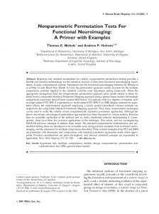
Results Type I Error Control The distributions of Type I error rate estimates for the four permutation methods and the WLS method, across all conditions examined in this study, are presented in as box-andwhisker plots in Figures 1 – 3 for nominal alpha levels of .01, .05, and .10, respectively. These figures reveal that all methods provided adequate control of Type I error rates (according to Bradley’s, 1978, liberal criterion) across the majority of conditions examined. However, these figures also suggest that for a subset of conditions, the tests showed excessively liberal or excessively conservative Type I error control. As expected, the degree of Type I error control increased as the nominal alpha level increased (that is, the tests are considered ‘robust’ in more conditions if nominal alpha is set at .05 than if nominal alpha is set at .01). Further, the typical deviation from nominal Type I error control associated with the WLS test in these conditions is that it became conservative rather than liberal. To identify the experimental design factors associated with changes in Type I error control, the proportions of conditions in which adequate control was demonstrated were calculated. The proportions were examined for each factor included in the Monte Carlo design (Table 1). At a nominal alpha level of .05, the WLS test showed more conditions with adequate control as the magnitude of the random effects variance, τ 2 , increased (with proportions ranging from .711 to .926). Variance heterogeneity in the primary studies had only a small impact on these proportions (.860 with homogeneous variances and .831 with a 1:4 variance ratio) and little impact was observed with either changes in the degree of correlation among the predictors or with distribution shape. Sample size, however, played a role in Type I error control, with better control evidenced as the number of studies included in the meta-analysis (k) increased and as the sample sizes in the primary studies (n1, n2) increased. Among the permutation tests, the Freedman and Lane and the Manly test provided the highest proportions of conditions with adequate Type I error control. For the Freeman and Lane test, the smallest of the marginal proportions was .993 (for the n1 =4, n2 = 6 conditions), while the Manly test did not drop below .997. In contrast, the Ter Braak test evidenced severe problems with Type I error control with k = 10 (maintaining adequate control in only 18.1% of the conditions.

Meta-Analytic Permutation Tests 11

0.10 0.09

Proportion of Rejections

0.08 0.07 0.06 0.05 0.04 0.03 0.02 0.01 0.00

WLS

Freedman & Lane

Kennedy

Manly

Statistical Test

Figure 1. Distributions of Type I Error Rate estimates for nominal α = .01

Ter Braak

Meta-Analytic Permutation Tests 12

0.25

Proportion of Rejections

0.20

0.15

0.10

0.05

0.00

WLS

Freedman & Lane

Kennedy

Manly

Statistical Test

Figure 2. Distributions of Type I Error Rate estimates for nominal α = .05

Ter Braak

Meta-Analytic Permutation Tests 13

0.25

Proportion of Rejections

0.20

0.15

0.10

0.05

0.00

WLS

Freedman & Lane

Kennedy

Manly

Statistical Test

Figure 3. Distributions of Type I Error Rate estimates for nominal α = .10

Ter Braak

Meta-Analytic Permutation Tests 14

Table 1 Proportion of Conditions with Adequate Type I Error Control (Bradley’s, 1978 Liberal Criterion) by Monte Carlo Design Factors.

α = .10

α = .05

α = .01

WLS

FL

KN

MN

TB

WLS

FL

KN

MN

TB

WLS

FL

KN

MN

TB

0.870 0.991 0.995

1.000 1.000 1.000

0.998 0.997 0.996

1.000 1.000 1.000

0.669 0.751 0.697

0.711 0.890 0.926

1.000 0.996 0.998

0.930 0.944 0.925

1.000 1.000 0.999

0.636 0.733 0.687

0.495 0.632 0.670

0.691 0.712 0.683

0.715 0.744 0.710

0.937 0.914 0.914

0.560 0.645 0.612

0.948 0.961

1.000 1.000

0.998 0.996

1.000 1.000

0.698 0.719

0.860 0.831

0.998 0.997

0.936 0.931

1.000 0.999

0.675 0.701

0.612 0.590

0.692 0.701

0.738 0.711

0.922 0.920

0.604 0.612

0.952 0.946 0.964

1.000 1.000 1.000

0.998 0.995 0.998

1.000 1.000 1.000

0.686 0.689 0.743

0.847 0.837 0.851

1.000 0.996 0.997

0.926 0.930 0.943

1.000 1.000 0.999

0.669 0.665 0.723

0.589 0.607 0.605

0.680 0.679 0.725

0.725 0.695 0.748

0.919 0.921 0.923

0.604 0.609 0.612

0.899 0.991 0.986

1.000 1.000 1.000

0.992 1.000 1.000

1.000 1.000 1.000

0.222 1.000 1.000

0.758 0.906 0.892

0.994 1.000 1.000

0.836 1.000 0.987

1.000 0.998 1.000

0.181 0.983 0.998

0.454 0.684 0.693

0.309 0.920 0.935

0.493 0.918 0.826

0.924 0.914 0.923

0.198 0.798 0.892

0.862 0.892 0.896 0.969 0.997 0.976 1.000 1.000 1.000

1.000 1.000 1.000 1.000 1.000 1.000 1.000 1.000 1.000

0.993 0.997 1.000 1.000 0.997 1.000 0.997 0.990 1.000

1.000 1.000 1.000 1.000 1.000 1.000 1.000 1.000 1.000

0.772 0.788 0.806 0.694 0.670 0.715 0.642 0.653 0.635

0.609 0.639 0.649 0.885 0.906 0.920 1.000 1.000 1.000

0.993 0.997 0.997 1.000 0.997 1.000 1.000 1.000 0.997

0.910 0.917 0.934 0.941 0.920 0.934 0.938 0.944 0.965

1.000 1.000 1.000 1.000 1.000 0.997 1.000 1.000 1.000

0.772 0.767 0.781 0.670 0.649 0.663 0.622 0.632 0.635

0.280 0.212 0.271 0.649 0.618 0.670 0.872 0.924 0.913

0.692 0.694 0.684 0.715 0.701 0.674 0.698 0.688 0.722

0.612 0.628 0.698 0.743 0.767 0.726 0.753 0.799 0.792

0.913 0.931 0.903 0.917 0.906 0.910 0.955 0.924 0.931

0.671 0.670 0.698 0.608 0.583 0.625 0.528 0.542 0.549

Distribution Shape ( Sk , Kr ) 0, 0 0.951 9.000 0.997 2, 6 0.957 9.000 0.997

1.000 1.000

0.690 0.727

0.850 0.841

0.998 0.998

0.936 0.931

0.999 1.000

0.673 0.703

0.603 0.598

0.684 0.709

0.733 0.716

0.909 0.933

0.576 0.640

τ2 0.1 0.5 1.0

σ 12 : σ 22 1:1 1:4

ρij 0.00 0.20 0.60

k 10 50 100

n1 , n2 4, 6 5, 5 6, 4 8, 12 10, 10 12, 8 40, 60 50, 50 60, 40

Meta-Analytic Permutation Tests 15

The marginal Type I error rates for each Monte Carlo design factor, at a nominal alpha level of .05, are presented in Table 2. These data illustrate the conservative nature of the WLS test (all averages are less than the nominal .05 level) and show that the average Type I error rate for this test increased as sample size increased and as τ 2 increased. These data also highlight the general conservative nature of the Ter Braak test. In contrast, the average Type I error rate for the Freedman and Lane test and for the Manly test remained very close to the nominal alpha level across all of the conditions examined. Table 2 Mean Type I Error Rates by Monte Carlo Design Factors (Nominal α = .05 ).

WLS

FL

KN

MN

TB

0.033 0.038 0.039

0.045 0.046 0.046

0.053 0.052 0.053

0.049 0.050 0.050

0.031 0.033 0.032

0.037 0.037

0.046 0.046

0.053 0.053

0.050 0.050

0.031 0.032

0.00 0.20 0.60

0.037 0.037 0.037

0.046 0.046 0.046

0.054 0.053 0.052

0.050 0.050 0.049

0.032 0.031 0.032

k 10 50 100

0.035 0.038 0.038

0.040 0.049 0.049

0.068 0.046 0.043

0.050 0.050 0.050

0.019 0.037 0.041

n1 , n2 4, 6 5, 5 6, 4 8, 12 10, 10 12, 8 40, 60 50, 50 60, 40

0.026 0.027 0.027 0.037 0.037 0.037 0.047 0.048 0.048

0.046 0.045 0.046 0.047 0.046 0.046 0.046 0.046 0.045

0.050 0.049 0.049 0.054 0.054 0.054 0.056 0.056 0.055

0.050 0.049 0.049 0.050 0.049 0.050 0.049 0.050 0.050

0.035 0.034 0.035 0.032 0.032 0.032 0.029 0.030 0.029

0.046 0.046

0.053 0.053

0.050 0.050

0.031 0.033

τ2 0.1 0.5 1.0

σ 12 : σ 22 1:1 1:4

ρij

Distribution Shape ( Sk , Kr )

0, 0 2, 6

0.037 0.037

Meta-Analytic Permutation Tests 16

Statistical Power Estimates Estimates of statistical power of the WLS test and the four permutation tests are presented in Table 3. To save space, power estimates are reported for only a subset of conditions, but these results are representative of the entire set of conditions for which one of the regressors was non-null. These results reveal the substantial power advantages of the WLS procedure over all of the permutation tests. For example, with a large effect size ( f 2 = 0.35), k = 50, and small samples, the power of the WLS test was .66. Among the permutation tests in this condition, the most powerful test was the Manly test, with power of only .20, less than one-third that of the WLS test. Despite the conservative control of Type I error evidenced by the WLS test, it was clearly the most powerful among the procedures examined.

Table 3 Estimated Power of Statistical Tests Under Selected Conditions with Nominal α = .05 (Equal Sample Sizes in Primary Studies, Homogenous Variances, and τ 2 = 0.50). f2

k

ni

WLS

FL

KN

MN

TB

0.15

10

5 10 50

0.06 0.10 0.13

0.05 0.06 0.07

0.08 0.11 0.10

0.06 0.08 0.09

0.03 0.02 0.02

50

5 10 50

0.37 0.55 0.69

0.11 0.15 0.18

0.10 0.15 0.19

0.11 0.16 0.19

0.05 0.04 0.04

100

5 10 50

0.66 0.83 0.94

0.14 0.19 0.26

0.11 0.18 0.26

0.13 0.19 0.27

0.05 0.05 0.02

10

5 10 50

0.09 0.13 0.19

0.06 0.07 0.09

0.10 0.12 0.14

0.09 0.09 0.12

0.03 0.03 0.02

50

5 10 50

0.66 0.81 0.90

0.19 0.24 0.32

0.18 0.24 0.33

0.20 0.24 0.32

0.06 0.04 0.04

100

5 10 50

0.92 0.99 1.00

0.25 0.42 0.51

0.21 0.40 0.51

0.24 0.41 0.51

0.06 0.06 0.04

0.35

Meta-Analytic Permutation Tests 17

Among the permutation procedures, the Ter Braak test evidenced notably lower power than the other three procedures (with power so low that the test appears to be a consistently poor choice). Among the other permutation tests, the Kennedy procedure was the most powerful for small values of k, but the differences between the Kennedy, Freeman and Lane, and Manly tests’ power estimates at larger k were always trivially small.

Discussion The results of this research demonstrate the general conservative nature of the WLS test in random effects meta-analysis. Surprisingly, the Type I error control was relatively unaffected by non-normality and variance heterogeneity in the primary studies. Such robustness is important for meta-analysis because meta-analysts are typically not able to directly check for violations of assumptions in primary studies. That is, violations of these assumptions are particularly pernicious in the meta-analytic context because meta-analysts must rely on details in the reports of primary studies to evaluate the tenability of these assumptions (Keselman, et al., 1998). The apparent robustness of the WLS test in random effects models was not seen in earlier work with fixed effects meta-analysis (Hogarty & Kromrey, 2003) in which the WLS test evidenced liberal Type I error control when assumptions were violated. The inclusion of the estimated random effects variance component in the estimation of the standard errors of the regression weights led to a conservative test, but a test that appears to be relatively resistant in the face of violations of the assumptions of normality and homogeneity of variance in the primary studies. Such an effect in random effects vs. fixed effects models was anticipated by Harwell (1997). Three of the four permutation strategies that have been developed in the context of multiple regression analysis evidenced superior Type I error control when they were applied in the context of random effects meta-analysis (i.e., weighting observations by the estimated sampling error of the effect size and the estimated random effects variance component). Among these procedures, the Manly (1997) and the Freedman and Lane (1983) evidenced the best Type I error control among the conditions examined. In terms of statistical power the Kennedy (1995) permutation strategy provided the greatest power with few studies in the meta-analysis (k = 10) and only trivial differences were seen among the three tests with larger numbers of studies.

Meta-Analytic Permutation Tests 18

However, the power of all of the permutation tests was notably smaller than that of the normal theory WLS procedure. Meta-analysis has become increasingly important for the synthesis of research results in a variety of fields, including education, the behavioral sciences and medicine. The accuracy of inferences derived from meta-analysis depends upon the appropriate application of statistical tools. As the use of meta-analytic methods becomes more commonplace, researchers must remain mindful of the limitations of certain estimates. The results of this study suggest that the WLS procedure evidences excellent robustness properties in random effects models, in contrast to its relatively poor performance in fixed effects meta-analysis. This research furnishes valuable information about the sensitivity of traditional tests used in meta-analysis and provides guidance regarding the choice of alternative methods.

Meta-Analytic Permutation Tests 19

References Anderson, M. J. & Robinson, J. (2001). Permutation tests for linear models. Australian Journal of Statistics, 43, 75 – 88. Anderson, M. J. & Legendre, P. (1999). An empirical comparison of permutation methods for tests of partial regression coefficients in a linear model. Journal of Statistical Computation and Simulation, 62, 271 – 303. Bradley, J.V. (1978). Robustness? British Journal of Mathematics and Statistics Psychology, 31, 144-152. Cooper, H. & Hedges, L. V. (1994). Handbook of research synthesis. New York: Russell Sage Foundation. Fern, E. F. & Monroe, K. B. (1996). Effect size estimates: Issues and problems in interpretation. Journal of Consumer Research, 23, 89-105. Field, A. P. (2001). Meta-analysis of correlation coefficients: A Monte Carlo comparison of fixedand random-effects methods. Psychological Methods, 6, 161 – 180. Fleishman, A. I. (1978). A method for simulating non-normal distributions. Psychometrika, 43, 521-532. Freedman, D. & Lane, D. (1983). A nonstochastic interpretation of reported significance levels. Journal of Business and Economic Statistics, 1, 292-298. Good, P. (1994). Permutation tests: A practical guide to resampling methods for testing hypotheses. Springer-Verlag, New York. Harwell, M. (1997). An empirical study of Hedges' Homogeneity Test. Psychological Methods, 2, 219-231. Hedges, L. V. (1994). Fixed effects models. In H. Cooper & L. V. Hedges (Eds.) Handbook of research synthesis. New York: Russell Sage Foundation. Hedges, L. V. & Olkin, I. (1985). Statistical methods for meta-analysis. Orlando, FL: Academic Press. Hedges, L. V. & Vevea, J. L. (1998). Fixed- and random-effects models in meta-analysis. Psychological Methods, 3, 486-504. Hogarty, K. Y. & Kromrey, J. D. (1999). Traditional and robust effect size estimates: Power and Type I error control in meta-analytic tests of homogeneity. American Statistical Association Proceedings of the Section on Government Statistics and Section on Social Statistics, 426-431.

Meta-Analytic Permutation Tests 20

Hogarty, K. Y. & Kromrey, J. D. (2003, April). Permutation tests for linear models in meta-analysis: Robustness and power under non-normality and variance heterogeneity. Paper presented at the annual meeting of the American Educational Research Association, Chicago. Kennedy, P. E. (1995). Randomization tests in econometrics. Journal of Business and Economic Statistics, 13, 85-94. Kennedy, P. E. & Cade, B. S. (1996). Randomization tests for multiple regression. Communications in Statistics: Simulations, 25, 923 – 936. Keselman, H. J., Huberty, C. J., Lix., L. M., Olejnik, S., Cribbie, R. A., Donahue, B., Kowalchuk, R. K., Lowman, L. L., Petoskey, M. D., Keselman, J. C., Levin, J. R. (1998). Statistical practices of educational researchers: An analysis of their ANOVA, MANOVA, and ANCOVA analyses. Review of Educational Research, 68, 350-386. Manly, B. F. J. (1997). Randomization, bootstrap and Monte Carlo methods in Biology (2nd Edition). London: Chapman and Hall. Oja, H. (1987). On permutation tests in multiple regression and analysis of covariance problems. Australian Journal of Statistics, 29, 91 – 100. Raudenbush, S. W. (1994). Random effects models. In H. Cooper & L. V. Hedges (Eds.) Handbook of research synthesis. New York: Russell Sage Foundation. Robey, R. R. & Barcikowski, R. S. (1992). Type I error and the number of iterations in Monte Carlo studies of robustness. British Journal of Mathematical and Statistical Psychology, 45, 283-288. Ter Braak, C. J. F. (1992). Permutation versus bootstrap significance tests in multiple regression and ANOVA. In K-H. Jockel, G. Rothe & W. Sendler (Eds.) Bootstrapping and related techniques, p. 79-86. Berlin: Springer-Verlag.