The Review of Regional Studies, Vol. 33, No. 1, 2003, pp. 104-120
Perplexity, Complexity, Metroplexity, Microplexity: Perspectives for Future Research on Regional Growth and Change* David A. Plane Department of Geography and Regional Development, University of Arizona Harvill Building, Box 2, Tucson, AZ 85721 USA, e-mail:
[email protected]
Abstract In this paper I make some summarizing comments regarding the papers in this special issue. I argue that we have entered a product-specialization stage in regional science scholarship and that there may now be a need for some broad synthesizing research such as that characteristic of earlier years of the research venture. I contend that studies of regional growth and development constitute “the highest form of the regional scientist’s art.” And I argue for greater consideration to be given to disaggregating our variables by demographics and paying greater attention to geographic units and scales. In that spirit, I present some information about the forthcoming new system of Core-Based Statistical Areas. I use an experimental version of the new system of Metropolitan and Micropolitan Statistical Areas to illustrate some urban-scale effects evident in recent county-level growth trends.
*
An earlier version was presented at the session “The Perplexing Literature: Regional Growth and Change: Conclusions and Perspectives for Future Research” at the 48th Annual North American Meetings of the Regional Science Association International, Charleston, South Carolina, November 16, 2001. I gratefully acknowledge the contributions of my doctoral student Christopher Henrie for his GIS and data-analysis assistance and the support of the U.S. Census Bureau, Population Division, for my sabbatical year research project in the Population Distribution Branch. Special thanks to Jim Fitzsimmons, Assistant Division Chief, and John Long, Chief, Population Division, for arranging my visiting status at the Bureau and to my colleagues in the Population Distribution Branch, Todd Gardner, Rodger Johnson, Paul Mackun, Petra Noble, Marc Perry, Mike Ratcliffe, Trudy Suchan, and Donna Defibaugh for their contributions to the project.
Plane / The Review of Regional Studies, Vol. 33, No. 1, 2003, pp. 104 - 120
105
1. INTRODUCTION It has been my experience that we eggheads are not very good at drawing out the bigger implications of a research literature. Nor are we especially skilled at setting broad agendas for future research. Usually when we are offered the opportunity to make such assessments, we pull a couple or three dripping wet studies out of the babbling brook of current research. These we proudly hold up (as if for the event-recording camera) as prototypes for the way things ought to be done henceforth. Posthaste. Or else we use the occasion as a happy excuse to tout our own current research fancies. I can’t promise that what I shall do herein will be all that different from standard practice. My conclusions for this suite of theme papers may well be part fish story (based on the new catches we’ve just been presented with in this issue) and, equally, part self-indulgence. 2. THE HIGHEST FORM OF THE REGIONAL SCIENTIST’S ART Alan Schlottmann, in dreaming up the idea for this assessment project, came up with the intriguing title: “The Perplexing Literature: Regional Growth and Change.” To start with, I would return to the question posed in the introductory paper: whether what we are talking about is even a single literature, or whether it is in fact an amalgamation of a number of different interwoven strands of research. Schlottomann and Bartik in their introduction make the pitch for at least a bifurcation of the research. They distinguish two broad strands of thought: one focused on general determinants of growth and one that seeks to identify public policy that impacts the growth process. I suspect there’s great heterogeneity within each of those two divisions. It strikes me that with as broad a topic as the regional science of growth and change we will always exhibit a tendency to scurry back into our own warm and familiar bailiwicks. Projects such as this one can be quite useful because they encourage us to pop our heads up from those prairie dog holes long enough to scout around and see what others, nearby, are doing. As the regional science research enterprise has matured, we’ve entered a product-specialization stage in our research venture; our analyses have become more focused, more technically sophisticated, but maybe also less conceptually broad-ranging than the research during the earlier, prototypedevelopment stage. Are we now in need of some synthesizing scholarship – the Bill Alonso, the Brian Berry, the Walter Isard style of work – that seeks to extract the big picture from among the tangles of the specialized literatures? In thinking about the role of the growth and change literature in regional science, my mind churned up a presidential address by John Fraser Hart to the Association of American Geographers back in 1981 (Hart 1982). Hart’s title was “The Highest Form of the Geographer’s Art.” That speech was a spirited defense of “old-fashioned” regional geography. It seems to me that researching regional growth and change is in some sense the highest form of the regional scientist’s art. In seeking to understand the multiplicity of causes for regional growth and decline in developed countries possessing highly interdependent urban systems, we engage ourselves in a quest fraught with extreme complexity if not perplexity. A full understanding may always lie beyond our grasp; a good partial one may depend on harmonizing a multiplicity of perspectives.
Plane / The Review of Regional Studies, Vol. 33, No. 1, 2003, pp. 104 - 120
106
The papers in this package blend themes in interesting ways; taken together I think we get the sense of classic regional science chamber music. Riddel and Schwer tackle a basic issue: what lies at the heart of generating growth? What changes economic history? What is it that sets in motion the swirling patterns that we try to track when we pour over variables measuring growth and change? What are the underlying incubating conditions that lead to innovation? Their take on the innovative “milieu” is a concept of “regional innovative capacity.” The type of model they use, in which current-period stocks of this elixir partially determine its future flows, has interesting similarities to traditional concepts of regional comparative advantage as expressed through the different types of economies of scale. Kim, Pickton, and Gerking tackle issues connected to another stimulus for growth and development: foreign direct investment. They make the point that FDI is inherently footloose: that, a priori, such outside interventions in local economies can be injected anywhere. Their data and analysis highlights, though, the role of existing and developing industrial specialization and inter-industry complexes. And they tackle rather head-on one of the big themes that runs throughout most of the growth literature: the role of agglomeration economies. They ask the question: can smaller economies partially offset location disadvantages through state financial incentives? Brown, Hayes, and Taylor also focus on policy instruments, seeking to expand our understanding of how state and local policies influence factor markets. Through their modeling they contest that policies more profoundly influence the private capital-to-labor ratio in a region than private output. West treats modeling issues. Two very interesting aspects of her article are: (1) the comparison of methodologies, traditions, and results between demographic population projections and revenue and other economic forecasts; and (2) the considerable attention she pays to the metropolitan scale of analysis. Too rarely have differing disciplinary practices for related growth and change problems been compared. And also too rarely have we focused on the functional geographic scale – the metropolitan region – at which so many of the locational decisions are made that determine aggregate growth and change at broader regional scales (such as the state level). I’m intrigued by her observation that in the case of population projections for Florida counties, demographic specialization matters, however economic functional specialization does not. To what extent is this true for the country as a whole? Quigley (1998) emphasizes the importance of economic diversity or heterogeneity for sustained city growth. His work focuses on the role of economies arising from: (a) shared inputs in production and consumption, (b) reduced costs from matching, and (c) reductions in variability – all of which increase with additional diversity of economic activities. Finally, in a provocative piece, Partridge and Rickman ask: “Do we know economic development when we see it?” They cogently point out that when examining sets of healthily developing regions or sets of lagging regions it is virtually impossible for all indicators to show their expected signs. Again, much of the discussion focuses on the optimal size of regional
Plane / The Review of Regional Studies, Vol. 33, No. 1, 2003, pp. 104 - 120
107
economies – a topic that has garnered immense amounts of attention in the regional science literature over the decades. Five very different yet complementary papers, all focused on different aspects, building from different foundational micro-economic underpinnings, but all contributing to the ongoing surge of results that over the last half century has perpetually replenished the cascading streams of regional science / regional economics / economic geography literature on growth and change. 3. REGIONAL DEVELOPMENT AND THE GEOGRAPHY OF CONCENTRATION Perhaps it would be instructive to go back in time to the beginning of the last half-century. The maps in Figures 1 and 2 illustrate county-level growth patterns in the U.S. during the 1950s and the 1990s.1 I pick the 1950s as our base for comparison for several reasons. For one thing, it was then that modern regional science was coming into existence: the statistical and theoretical modeling of regional economic phenomenon came to the fore with the establishment of the Regional Science Association and with Isard’s foundational work at the University of Pennsylvania. This time span also may be the approximate median life span of readers of this journal? While longer-term historical perspectives may indeed be revealing (we should probably set our work in the context of the sweep of history since the beginnings of the industrial revolution!), making sense of the trends witnessed during our own lifetimes is plenty perplexing. I also pick the 1950s as our jumping off point because a watershed in U.S. settlement patterns was then being reached. In 1958 Edward Ullman published his classic article in the Papers of the Regional Science Association titled "Regional Development and the Geography of Concentration" (Ullman 1958). In this paper he extolled the seeming inexorability of agglomerative advantages of the national core territory, which he identified as the American Manufacturing Belt plus Megalopolis. The trends extant during the 1950s can now be seen as precursors to the stronger deconcentration patterns soon to come about – note the evidence of strong westward movement and the rise of areas on the Gulf Coast and Florida in Figure 1. However, in the final years of the post-war decade, Ullman could still confidently proclaim the ongoing primacy of the core. With respect to the majority of the land area of the country outside the approximately 14-state core, he observed: In contrast to the core areas the prospects for the fringe or corner areas appear rather bleak, since they are remote from the center of the system and the self generating momentum of the center. Their best hope is to possess some special lure such as the present role of climate of California or Florida, or, in the past, the superior trees in the Pacific Northwest. Only by such lures have the corner areas been able to overcome their remoteness from the Industrial Belt… (Ullman 1958, p. 185).
1
The choropleth categories for both maps are based on the U.S. overall growth rate of 13.2 percent during the 1990s. The decadal growth rate for the 1950s was 18.5 percent.
Plane / The Review of Regional Studies, Vol. 33, No. 1, 2003, pp. 104 - 120
FIGURE 1 The County Level Geographic Pattern of Population Growth in the United States During the 1950s
FIGURE 2 The County Level Geographic Pattern of Population Growth in the United States During the 1990s
108
Plane / The Review of Regional Studies, Vol. 33, No. 1, 2003, pp. 104 - 120
109
In 1958 Ullman was not chary that amenities in the periphery could overcome the industrial complex advantages of the core despite having just four years earlier published a paper extolling their role (Ullman 1954). A half of a century later, growth and development trends are rather different. While we think we’ve by now gained a pretty strong handle on the geographic forces of industrialization and the attendant spatial growth trends set in motion in the mid-nineteenth century (the organizing principles of mass production and the corollary urbanizing logic of the industrial revolution), we remain less certain about today’s comparable trend setters and truly revolutionary regional economic forces. But we know a good deal. We know that capital is hugely more mobile and less placerooted. We appreciate that labor factors have risen to the fore, and these are more variegated than was previously the case. Regions’ human capital endowments are critical; but people, like capital, are fancifully more footloose than were their forebears. And we believe in a major role for natural amenities. (In fact, many of our regional science brethren derive considerable utility from hedonically pursuing their measurement and valuation.) So what perspectives are suggested for the research ahead? What I see is the need to bring both geography and demography more centrally into our analyses. 4. WHAT ABOUT PEOPLE AND WHAT ABOUT GEOGRAPHY IN REGIONAL SCIENCE? It has now been more than 30 years since Torsten Hägerstrand’s memorable presidential address to the Regional Science Association in which he asked the poignant question: “What about people in regional science?” (Hägerstrand 1970). More than ever I think his trumpet call is relevant to our future research agenda. For the kinds of questions we grapple with today in the growth and change literatures, a region’s population and its labor force cannot be treated as undifferentiated masses. No longer is it simply the age of mass production and mass consumption. Many growth industries are those that develop specialized products, seek out segmented markets, and engage in sophisticated analyses of marketing demographics. Similarly, for future regional growth research, productive synergies should be developed between demography and regional economics. Regional science is a good venue for economic/ demographic multidisciplinarity to flourish. And I’m a believer in the need for greater inputs of old-time economic geography into our theorizing. We need to be more sensitive to questions about geographic scale. We need to spend more time scrutinizing geographic patterns. And we need to attempt to relate our general research findings to the functional geographic structures in which the processes we study are played out. Several of the papers in this package focus on the state level of analysis: correctly so, given their interest in state-level policy variables. But the functional economic units of growth and change are extended metropolitan regions. Where are regional science’s current contributions to understanding these entities fundamental to current research?
Plane / The Review of Regional Studies, Vol. 33, No. 1, 2003, pp. 104 - 120
110
Beginning in the 1970s a veritable cottage industry developed involving the production of studies focused on the “metro-nonmetro turnaround” phenomenon. The debate was overly simplistic in drawing such a sharp dichotomy. Little research since Ravenstein’s 1885 seminal study of migration trends in Britain has sought to analyze streams of movement up and down the levels of the metropolitan hierarchy. Are the industrial-revolution-era patterns of step migration that Ravenstein documented – net flows of migrants inexorably up the urban hierarchy – still those relevant in today’s post-industrial societies? 5. METROPLEXITY AND MICROPLEXITY 5.1 The New System of Core-Based Statistical Areas In 2003 the most fundamental revision in the U.S. system of metropolitan-area delineation will be implemented. Under new Office of Management and Budget (OMB) approved standards (Federal Register 2000) we will soon have a nationwide system of CBSAs (core-based statistical areas). CBSAs will be inclusive of both Metropolitan Statistical Areas and Micropolitan Statistical Areas. Like the current MSAs, Metropolitan Statistical Areas defined according to the new standards will be composed of groups of counties centered on Urbanized Areas of 50,000 or more population. The new Micropolitan Statistical Areas will be built up from “Urban Clusters” having populations of 10,000 to 49,999. Urban Clusters are units analogous to Urbanized Areas in that they both delineate contiguous territory having high density of population. Collectively, Urbanized Areas and Urban Clusters are now in official OMB/Census Bureau parlance referred to as “Urban Areas.” I would like to close this call for renewed research on the functional economic and demographic nature of current metropolitan development by presenting some population growth statistics aggregated from the county-level rates shown in Figure 2 for the 1990s. These statistics are for what I am calling the “micropolitan/metropolitan spectrum,” a size-based classification I’ve based on the illustrative set of CBSAs published on the Census Bureau’s website in 1999 as part of the recent metropolitan standards review. The Metropolitan and Micropolitan Statistical Areas shown in Figure 3 are defined on 1990 rather than Census 2000 commuting data and on 1990 Urbanized Areas. Incorporated place boundaries rather than Urban Cluster boundaries were used to define principal cities for the Micropolitan Statistical Areas. The official CBSAs to be released by OMB in 2003 will differ somewhat from these experimental units delineated by the Geographic Distribution Branch of the Census Bureau. Changes in commuting patterns have taken place since 1990 that should result in some changes in the aggregation of outlying with central counties, and there will, of course, be differences between 2000 Urban Areas and their 1990 proxies. 5.2 Growth Rates by Size-Class Level Within the Micropolitan-Metropolitan Spectrum Table 1 shows growth rates calculated according to the different size classes of the micropolitan/metropolitan spectrum. Two columns of percentages are shown. The overall rate is an aggregate figure for all population living in counties classified at a particular hierarchical level; the mean rate is the average rate for all counties falling into a particular CBSA classification. For Metropolitan Statistical Areas, the mean county rates tend to be higher than
Plane / The Review of Regional Studies, Vol. 33, No. 1, 2003, pp. 104 - 120
111
the overall rates because (as we will see in more detail in a moment) outlying suburban counties are generally faster-growing than central counties (that is, counties encompassing the Urbanized Area cores). Central counties, however, account for overall majorities of total population. There is a clear size progression in terms of either set of growth rates. With two exceptions, the larger the CBSA unit, the faster the 1990–2000 rate of growth. An exception is for the country’s largest metropolitan areas—those which I have dubbed the “Mega” Metros. (These constitute an official class under the new OMB definitions: with Urbanized Area populations of 2.5 million or more, such MSAs qualify for subdivision into “Metropolitan Divisions.”) “Mega” Metros were growing notably more slowly than the next largest size class – “Major Metros” (those with more than 1 million total population but Urbanized Area cores of less than 2.5 million). Of course, as is always the case, percentage growth rates don’t tell the whole story. A relatively large share of national growth during the 1990s took place in the very largest metro areas despite the fact that they were growing less rapidly than the nation as a whole. The absolute increase of inhabitants attendant to an 11.3 percent growth rate in a single Mega MSA having a base of 10 million is more than that which would be accounted for by 20 percent growth taking place in 22 MSAs with population bases of 250,000. FIGURE 3 The “Micropolitan / Metropolitan Spectrum”: Experimental Core-Based Statistical Areas of the United States
Plane / The Review of Regional Studies, Vol. 33, No. 1, 2003, pp. 104 - 120
112
TABLE 1 Population Growth Rates Across the “Micropolitan/Metropolitan Spectrum,” 1990–2000 CBSA Classification All Counties Metropolitan Statistical Area Counties Mega Metro (UA pop. > 2.5 million) Major metro (MSA pop. > 1.0 million) AAA Metro (MSA pop. 500,000 − 999,999) AA Metro (MSA pop. 250,000 − 499,999) A Metro (MSA pop. < 250,000) Micropolitan Statistical Area Counties Non-CBSA Counties
Overall Pct. Rate 13.2 13.9 11.3 17.9 12.6 13.6 11.9 11.0 10.2
Mean Cty. Pct. Rate 11.2 18.1 20.0 25.6 15.9 15.9 12.9 10.1 7.7
No. of Counties 3,140 891 105 243 102 174 267 581 1,668
Speaking of metros of 250,000, the other break in the progressive sequence of growth rates with CBSA size is that for the “AA” category. Metropolitan areas of 250 thousand to half a million grew slightly faster overall than did those with between half and one million population. 5.3 Growth Rates by Central/Outlying Status How did counties fare across the “micropolitan/metropolitan spectrum” according to their suburban and exurban status? The new CBSA definitions contain rules distinguishing “central” and “outlying” counties based on strengths of commuting interaction and the amount of population included within the unit’s core – that is, its Urban Area core, be that an Urbanized Area for a Metropolitan Statistical Area or an Urban Cluster for a Micropolitan Statistical Area. Micropolitan Statistical Areas, however, are overwhelmingly single county units, so the central/outlying distinction is not particularly meaningful for them. In most instances commuting zones are contained within the same county as the Urban Clusters defined for micropolitan principal cities. In the case of the largest (“Mega”) Metropolitan Statistical Areas, a tripartite county classification is set forth in the OMB rules. Based on commuting ratios, this classification is for use in defining constituent “Metropolitan Divisions.” Table 2 shows growth rates bifurcated (or trifurcated) into central/outlying (or main/secondary/tertiary) county components. For all levels of the metropolitan spectrum the outermost counties grew faster than areas at the cores. No big surprise or change over previous decades trends there. 5.4 Growth Rates by Combined CBSA Status What may be of more interest is to look at the geographic positioning of Metropolitan and Micropolitan Statistical Areas within the overall urban system. That is, to examine not only a county’s own CBSA classification, but also that county’s proximity to other CBSAs. The new definitions pay some attention to such functional nesting. Provisions allow for Metropolitan and Micropolitan Statistical Areas to form a separate tier of combined areas in cases where there are moderately strong commuting ties, but the ties are not strong enough to qualify the areas to merge into a single unit. Whereas the basic rule for assigning an outlying county to a CBSA is a
Plane / The Review of Regional Studies, Vol. 33, No. 1, 2003, pp. 104 - 120
113
25 percent commuting tie to the central county or counties of the CBSA,2 two or more CBSAs can form a ‘Combined Statistical Area’ if they have an employment interchange measure (sum of bi-directional flows) of 15 percent or more.3 Note that any combination of micropolitan and metropolitan areas may cluster together in a Combined Statistical Area. Under several earlier sets of standards for metropolitan area definition only the largest metroplexes were recognized as interconnected entities called Consolidated Metropolitan Statistical Areas (CMSAs). Table 3 shows growth rates for counties lying within the experimental Core Based Statististical Areas at different levels of the “micropolitan/metropolitan spectrum” split out by their “combined status.” I define combined status to be the highest level of the spectrum represented by the CBSAs included within the combined statistical area. Laramie, Wyoming and De Kalb, Illinois both qualify as Micropolitan Statistical Areas. However, these two areas are situated quite differently within the country’s urban system. According to the experimental CBSA classifications, the De Kalb Micropolitan Statistical Area combines with the Chicago Mega-Metropolitan Statistical Area, whereas Laramie does not qualify to combine with any other unit – even the (adjacent) “Class–A” Cheyenne Metropolitan Statistical Area. How might a county’s combined status affect the growth rate it could expect based simply on its hierarchical level within the micropolitan/metropolitan spectrum? Much attention in the growth literature has been given to spread and backwash effects (Gaile 1980). Focusing on combinations up the size hierarchy recognizes that smaller Core-Based Statistical Areas positioned within major metropolitan conurbations may benefit from greater agglomeration economies (spread effects) than similarly sized areas situated outside the commuting ranges of large metropolitan areas. This would lead us to predict faster growth for counties in such TABLE 2 Population Growth Rates for Central and Outlying Counties of Experimental Metropolitan Statistical Areas, 1990 –2000 Metropolitan Classification
Mega Metro (UA pop. > 2.5 million)
Major Metro (MSA pop. > 1.0 million) AAA Metro (MSA pop. 500,000 − 999,999 AA Metro (MSA pop. 250,000 − 499,999) A Metro (MSA pop. < 250,000) 2
Overall Pct. Rate
Mean Cty. Pct. Rate
No. of Counties
Main
Secdry
Tertry
Main
Secdry
Tertry
Main
Secdry
Tertry
9.0
10.6
19.0
10.0
13.4
28.3
21
33
51
Central
Outlying
Central
Outlying
Central
Outlying
17.5
29.4
22.9
31.4
167
76
12.2
25.4
13.0
24.4
76
26
13.3
17.9
14.1
20.2
121
53
11.7
16.9
11.5
17.2
198
69
Either 25 percent of the outlying county’s employed residents must “in” commute to the central county or counties or 25 percent of the employment in the outlying county must be accounted for by workers “out” commuting from the central county or counties. 3 The combination is automatic if the sum of the flows in both directions is 25 percent or more; local opinion (as expressed through the Congressional delegations from the affected state or states) will determine whether a combination takes place in cases where the exchange measure lies in the 15 to 25 percent range.
Plane / The Review of Regional Studies, Vol. 33, No. 1, 2003, pp. 104 - 120
114
TABLE 3 Population Growth Rates by Combined Status Across the “Micropolitan/Metropolitan Spectrum,” 1990-2000 County CBSA Classification Combined Status Major Metro (MSA pop. > 1.0 million) Mega-Metro Combined Not Mega-Metro Combined AAA Metro (MSA pop. 500,000 − 999,999) Mega-Metro Combined Major-Metro Combined Major or Mega Combined Not Major or Mega Combined AA Metro (MSA pop. 250,000 − 499,999) Mego-Metro Combined Major-Metro Combined AAA-Metro Combined AAA or Above Combined Not AAA or Above Combined A Metro (MSA pop. < 250,000 Mega-Metro Combined Major-Metro Combined AAA-Metro Combined AA-Metro Combined AA or Above Combined Not AA or Above Combined Micropolitan Mego-Metro Combined Major-Metro Combined AAA-Metro Combined AA-Metro Combined A−Metro Combined Metropolitan Combined Not Metropolitan Combined
Overall Pct. Rate
Mean Cty Pct. Rate
No. of Counties
20.8 17.7
21.6 25.6
3 240
8.5 12.2
9.0 10.5
7 3
9.5 13.3
9.4 16.6
10 92
12.4 29.3 25.1
11.7 29.3 26.1
7 1 6
16.7 13.2
19.1 15.7
14 160
13.8 10.9 13.2 12.7
12.9 12.2 11.9 12.2
5 5 7 10
12.7 11.8
12.3 13.0
27 240
12.6 19.0 8.1 20.9 11.0
12.5 16.4 9.6 19.3 8.6
11 40 20 23 31
15.3 9.3
13.6 9.2
125 456
Combined Statistical Areas as opposed to those in “stand-alone” metros. Alternatively, however, smaller CBSAs may experience negative urban shadow (or backwash) effects from being situated near larger metropolises. They may not develop some of the functionality that would exist were they to be the main central place for an extensive hinterland region. From this consideration we would predict slower growth for the combined than the stand-alone metropolitan area. So, does one or the other of these opposing considerations predominate? And does it depend on level within the micropolitan/metropolitan spectrum? Evidence in Table 3 is hardly definitive. It does suggest, however, that for AAA–Metros (those from 500,000 to 999,000 in population) growth seems to be retarded by being within the
Plane / The Review of Regional Studies, Vol. 33, No. 1, 2003, pp. 104 - 120
115
extended commuting field of major MSAs (those of 1 million or more population). For micropolitan areas, it seems clear that being combined with a metropolitan area results in higher probabilities for rapid growth. There don’t seem to be strong differences for combined or noncombined status among A–Metros and AA-Metros or for the million-person-or-greater Major Metro Areas. Note, however, that the sample sizes for many of the combined status categories are quite small. 5.5 Growth-Rate Effects Within Extended Metropolitan Hinterlands: A Proximity-Class Approach Doubtless the economic influence of metropolitan areas extends well outside the boundaries of the relatively strong commuting fields recognized by the new Combined Statistical Area criteria. It seems desirable to focus research on functional measures of metropolitan influence other than the journey-to-work. Unfortunately data are not collected countrywide for other types of daily urban people movements such as shopping and social trips. Television-channel viewing patterns become less and less relevant in the cable-channel/satellite-dish age, as do newspaper circulation zones due to the loss of many city dailies and the advent of national distribution systems. Telephone call patterns and perhaps certain classes of commodity flows may merit consideration. In the absence of compelling linkage data, a number of studies have examined simple county adjacency measures in order to detect spread and backwash effects. For example, Khan, Orazem, and Otto (2001) find that for an eight-state midwest study area local county population change responds positively to own-county economic growth, to economic growth in adjacent counties, and to growth two counties away, however the effect turns negative beyond a threecounty radius. Because of the irregular shapes of counties and their widely varying sizes in different states, rather than using adjacency, we prefer to study proximity classes based on GIS-calculated buffers around the urbanized core territory of the experimental CBSAs. Our approach is similar to the distance measurements used at the Census Tract level in the study by Henry, Barkley, and Bao (1997) of rural growth trends in metropolitan hinterlands in the south. Their modeling work, involving extensions to models developed in Carlino and Mills (1987) and, within an intrametropolitan context, Boarnet (1994), detected a mix of spillover (spread) and backwash effects from urban core areas to their rural hinterlands. Whereas Henry, Barkley, and Bao explicitly focused on rural areas proximate to metropolitan ones, our proximity concept is a more general one. Our analysis is based on assignment of counties in each micropolitan/metropolitan spectrum level to the higher-level CBSA buffer zones in which their geographic centers lie. We presumed that larger CBSAs had larger fields of influence, and we engaged in considerable experimentation with different buffering ranges. The county proximity classes used here are those based on buffers extending 50 miles from the geographic center of the principal city or cities that constitute the cores of Micropolitan Statistical Areas; 50 miles measured from the outer edges of the Urbanized Areas for Class–A, Class–AA, and Class–AAA Metropolitan
Plane / The Review of Regional Studies, Vol. 33, No. 1, 2003, pp. 104 - 120
116
Statistical Areas; 75-miles from UA boundaries for Major MSAs; and 100-miles from UA edges for Mega MSAs. In assigning counties to CBSA proximity classes (which we immodestly dub “Plane-Henrie Codes”), higher-level buffers take precedence over lower-level ones, as illustrated in Figures 4 and 5.4 There may be multiple layers in the nesting of these buffers. For instance consider the Plane-Henrie Code proximity classification of Rock County, Wisconsin, one of many complex cases found in the regional detail maps of Figure 5. The county itself is coterminous with the Class-A Janesville, WI Metropolitan Statistical Area. The City of Beloit and its environs on the county’s southern border, however, are actually part of the Urbanized Area of the Class-AA Rockford, IL Metropolitan Statistical Area, plus the county’s center lies within the 50-mile AA-buffer zone around this UA. It is also within the 50-mile AAFIGURE 4 “Plane-Henrie Code” Classification of County Micropolitan / Metropolitan Proximity
4
In the case of a few very large counties, a county’s geographic center may lie outside the buffer of its own CBSA’s urban area or of the urban-area buffer of the higher-level CBSA with which its metro area combines. In such cases, if the provisional proximity class calculated from all buffers is (a) lower than the hierarchy level of the CBSA that contains the county, and/or (b) lower than the combined status of the county, the higher of the county’s hierarchy class and combined status is assigned as its Plane-Henrie Code proximity class. Example 1: A county is the central county of a micropolitan area that combines with a metropolitan area in the AAA size class; however, its center lies outside all proximity buffers. It is assigned the Plane-Henrie Code: “Micropolitan, AAA-Metro Proximate.” Example 2 (Riverside County, California): A central county of a Major Metro Area combines with a Mega Metro Area. The county’s geographic center, however, lies outside the buffers of the urban areas of all CBSAs. It is assigned the Plane-Henrie Code: Major Metro, Central, Mega-Metro Proximate.
Plane / The Review of Regional Studies, Vol. 33, No. 1, 2003, pp. 104 - 120
117
buffer of the Madison, WI Urbanized Area. Additionally the county’s center lies within the 75mile buffer of the Milwaukee–Waukesha–West Allis, WI area, which we rank as a Major-Level Metro. But, all these considerations are trumped by the fact that the county also lies within the 100-mile buffer of a Mega Metro: the Chicago–Gary–Naperville, IL-IN MSA. Rock County is thus assigned the Plane-Henrie Code for “A–Metro, Central, Mega-Metro–Proximate” territory. The more general point is this: while in our central-place theories we’ve so painstakingly and lovingly detailed considerations of nested hierarchies of urban zones of influence, very rarely have these concepts been applied in migration analysis – which is one of the multiple literatures on regional growth and change. (For an exception, however, see Plane, Henrie, and Perry 2002.) Table 4 shows population growth rates for all the various assignments of counties to the Plane-Henrie proximity Codes. Unlike with the combined-status analysis, there are at least moderately large numbers of counties falling into each of the proximity classes. For large metropolitan areas – those in the Major and AAA categories – urban-shadow, growth-depressing effects appear to predominate over broad regional external economies of agglomeration, growth-enhancing effects. Major Metro counties more than 100 miles away from the Urbanized Area boundary of a Mega Metro had higher growth rates than did those that are proximate to a Mega area’s UA. And AAA Metro counties not proximate to Mega or Major Metros had faster growth than did counties whose centers lie within the 100-mile Mega-Metro or 75-mile Major-Metro buffers. FIGURE 5 Regional Detail Map of “Plane-Henrie Code” Classification of County Micropolitan / Metropolitan Proximity Showing the Underlying Overlapping Hierarchy of Urban-Area Proximity Buffers
Plane / The Review of Regional Studies, Vol. 33, No. 1, 2003, pp. 104 - 120
118
TABLE 4 Population Growth Rates by Plane-Henrie Code Proximity Classes Across the “Micropolitan/Metropolitan Spectrum,” 1990-2000 County CBSA Classification Proximity Class Major Metro (MSA pop. > 1.0 million) Mega-Metro Proximate Not Mega−Metro Proximate
Overall Pct. Rate
Mean Cty. Pct. Rate
No. of Counties
13.5 19.3
16.3 27.6
45 198
6.5 14.6
5.5 17.9
30 22
9.1 17.3
10.7 21.3
52 50
10.5 18.6 18.9
10.7 20.1 21.1
35 31 17
14.5 12.3
16.3 15.6
83 91
9.8 13.0 11.5 13.1
11.6 14.8 10.3 12.6
40 72 15 23
11.8 12.1
13.1 12.7
150 117
8.7 12.7 12.7 13.7 7.8
9.4 12.0 12.0 11.7 6.6
74 155 38 60 72
11.2 10.3
10.5 9.2
399 182
Non-CBSA Mega-Metro Proximate Major-Metro Proximate AAA-Metro Proximate AA-Metro Proximate A-Metro Proximate Micropolitan Proximate
13.2 12.8 15.3 10.3 8.7 5.4
12.8 12.9 13.2 9.5 6.7 3.2
121 287 58 187 231 355
Metropolitan Proximate CBSA Proximate Not CBSA Proximate
11.7 10.5 8.7
10.6 8.5 5.4
884 1,239 429
AAA Metro (MSA pop. 500,000 − 999,999) Mega-Metro Proximate Major-Metro Proximate Major or Mega Proximate Not Major or Mega Proximate AA Metro (MSA pop. 250,000 − 499,999) Mega-Metro Proximate Major-Metro Proximate AAA-Metro Proximate AAA or Above Proximate Not AAA or Above Proximate A Metro (MSA pop. < 250,000) Mega-Metro Proximate Major-Metro Proximate AAA-Metro Proximate AA-Metro Proximate AA or Above Proximate Not AA or Above Proximate Micropolitan Mega-Metro Proximate Major-Metro Proximate AAA-Metro Proximate AA-Metro Proximate A-Metro Proximate Metropolitan Proximate Not Metropolitan Proximate
For Micropolitan counties and counties outside all CBSA boundaries the opposite tendencies are clearly evidenced. Micropolitan counties that are proximate to AA and higher-level Metropolitan Statistical Areas grew faster than non-proximate micropolitan counties. An interestingly counter-point, however, is that Micropolitan Statistical Areas proximate to the
Plane / The Review of Regional Studies, Vol. 33, No. 1, 2003, pp. 104 - 120
119
smallest metropolitan areas – Class A Metros (those having less than 250,000 population) – grew more slowly than did non-proximate Micropolitan Statistical Areas. A probable reason is that micros and Class A Metros provide some of the same functions resulting in there being an urbanshadow effect on micropolitan areas proximate to Class-A metropolitan areas. A very similar pattern is found for the non-CBSA counties’ Plane-Henrie code classification. Non-CBSA counties proximate to A-level and above metropolitan areas grew faster than the most remote non-proximate non-CBSA counties. On the other hand, non-CBSA counties within 50 miles of a micropolitan principal city had lower growth rates on average than did the most remote nonCBSA counties. Evidently the presence of a nearby micropolitan area takes away some of the economic functions and some of the growth potential that might otherwise be endogenous to a non-CBSA county. 6. CONCLUSIONS The four dripping wet tables I’ve dredged up here are suggestive of the kind of research I envision completing in the next several years on migration patterns across the micropolitan/ metropolitan spectrum. Functional economic specialization as well as demographic classifications of the CBSAs will play a role in my attempts to understand hierarchical patterns of growth and movement. These as well as other broad avenues now extant in this perplexing literature seem promising routes to push frontierward as we continue to seek answers about the evolving geographic patterns and driving economic forces of regional growth and change. Perplexity, complexity, metroplexity, microplexity: the literature on regional growth and change developed over the last half-century has plenty of “exities.” I expect in the next half century that this ever-growing literature will continue to fascinate and frustrate. With a research area as complex as regional growth and change it is ultimately necessary to understand the demographic and geographical milieux in which development processes take place. People and geography really do matter for regional science. The topics highlighted in this set of papers provide scholars with a plethora of ongoing opportunities to indulge in the “highest form of the regional scientist’s art.” REFERENCES Boarnet, M.G., 1994. “An Empirical Model of Intrametropolitan Population and Employment Growth,” Papers in Regional Science 73, 135–153. Carlino, G.A. and E.S. Mills, 1987. “The Determinants of County Growth,” Journal of Regional Science 27, 39–54. Federal Register, 2000. “Standards for Defining Metropolitan and Micropolitan Statistical Areas; Notice.” December 27. Part IX: Office of Management and Budget 82, 228–82, 238. Gaile, G.L., 1980. “The Spread-Backwash Concept,” Regional Studies 14, 15–25. Hägerstrand, T., 1970. "What about People in Regional Science?" Papers of the Regional Science Association 25, 7–21.
Plane / The Review of Regional Studies, Vol. 33, No. 1, 2003, pp. 104 - 120
120
Hart, J.F., 1982. "The Highest Form of the Geographer's Art," Annals of the Association of American Geographers 72, 1–29. Henry, M.S., D.L. Barkley, and S. Bao, 1997. “The Hinterland’s Stake in Metropolitan Growth: Evidence from Selected Southern Regions,” Journal of Regional Science 37, 522–524. Khan, R., P.F. Orazem, and D.M. Otto, 2001. “Deriving Empirical Definitions of Spatial Labour Markets: The Roles of Competing Versus Complementary Growth,” Journal of Regional Science 41, 735–756. Plane, D.A., C. Henrie, and M. Perry, 2002. “Migration across the Micropolitan / Metropolitan Spectrum.” Paper presented at the 42nd Annual Meeting of the Western Regional Science Association, Monterey, California. Quigley, J.M., 1998. “Urban Diversity and Economic Growth,” Journal of Economic Perspectives 12, 127–138. Ravenstein, E. G., 1885. “The Laws of Migration,” Journal of the (Royal) Statistical Society 48, 167–227. Ullman, E. L., 1954. “Amenities as a Factor in Regional Growth,” Geographical Review 44, 119–132. Ullman, E.L., 1958. "Regional Development and the Geography of Concentration." Papers of the Regional Science Association 4, 179–198. Reprinted in J. Friedman and W. Alonso (eds.), Readings in Regional Development. MIT Press: Cambridge, MA, 1964, pp. 153–172; and in Bobbs-Merrill Reprint Series in Geography, 1968.